대회 소개
TGS Salt Identification Challenge
Segment salt deposits beneath the Earth’s surface
https://www.kaggle.com/c/tgs-salt-identification-challenge/overview
Description
Several areas of Earth with large accumulations of oil and gas also have huge deposits of salt below the surface.
But unfortunately, knowing where large salt deposits are precisely is very difficult. Professional seismic imaging still requires expert human interpretation of salt bodies. This leads to very subjective, highly variable renderings. More alarmingly, it leads to potentially dangerous situations for oil and gas company drillers.
To create the most accurate seismic images and 3D renderings, TGS (the world’s leading geoscience data company) is hoping Kaggle’s machine learning community will be able to build an algorithm that automatically and accurately identifies if a subsurface target is salt or not.
패키기 불러오기
1 | |
1 | |
데이터 불러오기
1 | |
1 | |
| id | rle_mask | |
|---|---|---|
| 0 | 575d24d81d | NaN |
| 1 | a266a2a9df | 5051 5151 |
| 2 | 75efad62c1 | 9 93 109 94 210 94 310 95 411 95 511 96 612 96... |
| 3 | 34e51dba6a | 48 54 149 54 251 53 353 52 455 51 557 50 659 4... |
| 4 | 4875705fb0 | 1111 1 1212 1 1313 1 1414 1 1514 2 1615 2 1716... |
| ... | ... | ... |
| 3995 | 9cbd5ddba4 | NaN |
| 3996 | caa039b231 | 2398 7 2499 11 2600 16 2700 22 2801 26 2901 29... |
| 3997 | 1306fcee4c | NaN |
| 3998 | 48d81e93d9 | 2828 1 2927 3 3026 5 3126 6 3225 8 3324 10 342... |
| 3999 | edf1e6ac00 | NaN |
4000 rows × 2 columns
1 | |
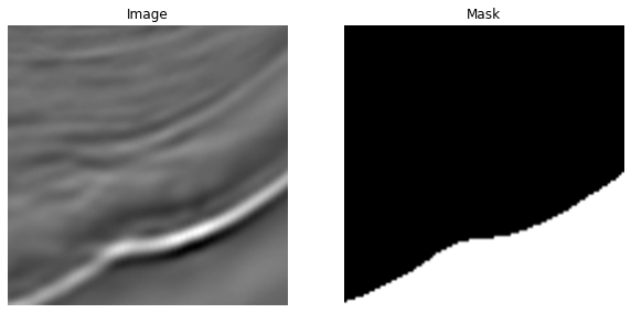
이미지(원본 및 마스크) 확인하기
1 | |
| images | masks | |
|---|---|---|
| 0 | ./train/images/46f402dcd5.png | ./train/masks/46f402dcd5.png |
| 1 | ./train/images/a56e87840f.png | ./train/masks/a56e87840f.png |
| 2 | ./train/images/2af3c055b2.png | ./train/masks/2af3c055b2.png |
| 3 | ./train/images/7c61d788af.png | ./train/masks/7c61d788af.png |
| 4 | ./train/images/ef654c1b73.png | ./train/masks/ef654c1b73.png |
| ... | ... | ... |
| 3995 | ./train/images/14152a6731.png | ./train/masks/14152a6731.png |
| 3996 | ./train/images/418b7878a8.png | ./train/masks/418b7878a8.png |
| 3997 | ./train/images/106e4043ba.png | ./train/masks/106e4043ba.png |
| 3998 | ./train/images/bce104494c.png | ./train/masks/bce104494c.png |
| 3999 | ./train/images/27a240a570.png | ./train/masks/27a240a570.png |
4000 rows × 2 columns
1 | |
데이터 전처리
segmentation대회의 정답값은 예전classification대회처럼 클라스 값이 아니라 이미지이다.- Input image에서 소금인 영역을 찾아내야 한다.
-
따라서 예전처럼
ImageDataGenerator로 데이터를 처리하기 까다롭기 때문에 직접 데이터셋을customizing해보자. segmentation에서는UNet모델을 가장 많이 사용한다.- 모델을 직접 쌓아보면 알겠지만 이미지의 사이즈가 2의 거듭제곱 형태이면 편하다.
- U 형태로 feature extraction이 이루어지고, 밑으로 갈수록 이미지의 크기는 작아지지만 채널 수가 늘어나는 특징이 있다.
- 이진분류, 다중분류 등에 사용된다.
Train Dataset 전처리하기
-
대부분
ImageDataGenerator로 이미지 전처리가 가능하지만, 몇몇 대회에선 이미지 형태에 따라 전처리를 직접 해야하는 경우가 있다. 어떤한 데이터 형태든 다룰 수 있도록 직접 전처리 하는 방법들을 익혀두자. -
먼저 데이터를 담을 빈 그릇을 만든다.
- 빈 그릇을 만들 때 너비, 높이 뿐만 아니라 채널을 잊지 말고 설정해주자.
- 이미지의 RGB 픽셀 값들을 보면 모두 같음을 알수 있다. 학습 속도 향상을 위해 하나의 채널만 사용하자.
- image 데이터 타입은 가장 효율적으로 정보를 담을 수 있는
dtype = np.uint8으로 설정한다.- 양수만 표현 가능하다.
- 2^8 개수 만큼 표현 가능하다.(0 ~ 255)
- y 데이터 타입은
dtype = np.bool로 설정한다.
1 | |
1 | |
빈 그릇 만들기
1 | |
이미지 데이터 담기
1 | |
Mask 데이터 담기
- Mask 데이터는 True, False 형태로 픽셀값이 채워져야 한다.
1 | |
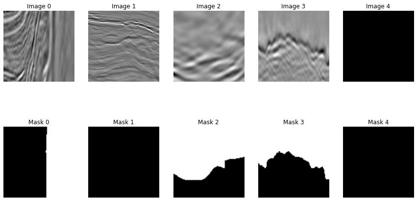
Train, Valid 나누기
segmentation은 회귀 문제의 느낌이 있다.- 이미지마다 소금이 들어있는 정도가 다를 수 있으므로, 회귀에서
y의 비율을 맞추려면 어떻게 해야할까.- 소금의 비율 구간을 나눈다.
- 구간별로 추출하면 안정적인 평가 셋이 될 것이다.
- 지금은 우선
train_test_split으로 일괄적으로 나누자.
1 | |
U-net 모델 구축하기
- Classification 문제에선 주로
model = Sequential()을 사용한 비교적 단순한 모델 구조를 쌓았다. -
함수를 이용하여 층들을 병렬로 쌓을 수 있는 방법을 적용하자.
Functional API라고도 부른다. - U-net 모델 구조의 특징
- 출력값의 크기는 Input의 크기와 같다.
- 이미지 분류 문제에서는 이미지의 크기가 작아지다가 Dense층을 거쳐 확률값으로 나가는 형태인데, Segmentation 문제에서는 input과 output이 똑같은 크기를 갖는다.
- 각각의 픽셀값이 [0,1] 사이로 출력 되어야 한다.
- 출력값의 크기는 Input의 크기와 같다.
가장 단순한 U-net 구조
- UNet에서는 padding 옵션 넣어 이미지의 크기가 줄어드는 것을 방지한다. 기본값인
valid이면 이미지 크기가 작아진다. - 0~1 사이로 값이 나가야하므로 출력층에서
sigmoid를 적용한다. - 모델을 선언할 때
input,output을 명시해준다.
1 | |
1 | |
U-net 구조 응용하기
-
Conv2DTranspose()층은 줄어든 이미지를 다시 키우기 위한 연산 작업이다. 비선형 학습이 이루어지지 않기 때문에activation함수를 설정해주지 않는다. concatenate를 통해 사이즈가 같은 층끼리 합쳐준다. 기본적으로axis=-1로 설정되어 있어 마지막 축을 기준으로 합쳐진다.- 아직은 U-net 구조를 깊게 쌓지 않아서 모델의 성능이 높게 나오진 않는다. 다른 하이퍼파라미터 최적화를 끝낸 후, 모델을 더 깊게 쌓아보자.
1 | |
1 | |
1 | |
1 | |
1 | |
Validation Data를 Mean IOU로 평가하기
- 대회 점수를 올리기 위해 다음의 과정을 거치게 된다.
- (1) 현재의 모델을 최적화하기
- (2) 모델의 구조를 복잡하게 하기
-
먼저 주어진 모델을 최적화한 다음 모델 구조를 복잡하게 해야 최소한의 노력, 시간으로 효율적으로 모델 성능을 높일 수 있다.
- Test 데이터셋을 예측하기 전, 이 대회의 평가 지표인
Mean IOU로 모델의 성능을 최적화 해보자.
Validation Dataset 크기 조정하기
1 | |
1 | |
Mean IOU채점 방식 역시 101x101 기준으로 이루어지기 때문에, 이와 같은 조건으로 설정해야 한다.- result_valid 및 y_valid의 크기를 바꿔주자.
1 | |
1 | |
1 | |
1 | |
Mean IOU 계산하기
-
validation dataset을 이용해 어떤
threshold값이 높은 mean IOU 값을 갖는지 확인하자. 적절한threshold를 찾아 Test Dataset 예측에 적용한다. threshold값을 높게 잡으면 보수적으로 예측하게 되어 실제 환자를 건강하다고 예측하는 경우가 발생한다.-
따라서 의료계에서는 보통
threshold을 낮게 잡는다. np.linspace(0,1,num)함수를 이용하여 0~1 사이를 num개의 간격으로 나누자.
1 | |
1 | |
1 | |
1 | |
1 | |
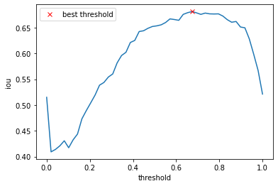
최적의 threshold 값 찾기
- threshold 별로 계산된 IOU 값을 시각화해보자.
- 최적의 threshold 값을
threshold_best에 저장하여 test data 예측에 사용한다. - 실제 제출 점수와 최적의 IOU 값이 비슷해야 모델이 안정적으로 학습된 것이다.
1 | |
1 | |
1 | |
1 | |
1 | |
1 | |
1 | |
1 | |
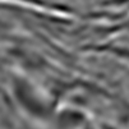
Test data 예측하기
- Train data를 구축했던 것처럼 Test data 역시 같은 방식으로 전처리 해주자.
model.predict()후 원래 이미지 크기인101x101로 resize 해줘야 한다.- 또한
np.squeeze()를 사용하여 마지막 차원을 제거해준다. 이미지의 차원도 다시 맞춰줘야 한다.
1 | |
1 | |
1 | |
1 | |
Submission 완료하기
-
segmentation대회에서는 보통 각 픽셀별로 확률값 자체를 제출하지 않는다. 지금 이 대회만 보더라도 이미지 하나에 101x101 = 10201개의 픽셀이 존자하고, 총 18000개의 테스트 이미지로 183618000 개의 확률값이 나오게 된다. 이 값들을 그대로 재출 시 엄청난 양의 연산이 채점에 필요하게 될 것이므로, kaggle 측에서는 보통 대회와는 조금 다른 제출 방식을 요구하고 있다. -
run-length encoding로 픽셀 값들을 바꿔준 뒤 제출을 해야 자신의 점수를 제대로 확인할 수 있다.- (1) 기본적으로
0.5보다 확률값이 높으면 1, 아니면 0으로 바꿔주자.0.5역시 하이퍼파라미터로, 최적의 값을 찾아줘야 한다.
- (2) 픽셀 값들을
run-length encoding로 바꿔준다. 1의 시작점과 시작점부터 run-length의 값이 한 쌍이 된다.- 예를 들어, 000111001111 의 픽셀 값은
3 3 8 4로 표현된다.
- 예를 들어, 000111001111 의 픽셀 값은
- (1) 기본적으로
Run-Length Encoding 함수
- run-length encoding 함수를 정의하고, 추출된 예측값을 dictionary 형태로 저장한다.
- dictionary로 저장시, key값은 test image의 주소, value 값은 run-length 인코딩된 값이다.
1 | |
1 | |
1 | |
최종 제출
- 기존의 제출 형식(칼럼 이름, 각 칼럼에 들어가는 값)을 확인하자.
- Dictionary 형태로 만들어둔 result 값을 제출 형식에 맞게 변형한다.
1 | |
| id | rle_mask | |
|---|---|---|
| 0 | 155410d6fa | 1 1 |
| 1 | 78b32781d1 | 1 1 |
| 2 | 63db2a476a | 1 1 |
| 3 | 17bfcdb967 | 1 1 |
| 4 | 7ea0fd3c88 | 1 1 |
| ... | ... | ... |
| 17995 | c78063e0a6 | 1 1 |
| 17996 | bfcdcd2720 | 1 1 |
| 17997 | 07c3553ef7 | 1 1 |
| 17998 | 9c2e45bf79 | 1 1 |
| 17999 | 41d0f0703c | 1 1 |
18000 rows × 2 columns
1 | |
| id | rle_mask | |
|---|---|---|
| 0 | ca0030c4ed | 46 7 103 1 106 1 149 6 204 1 207 1 249 6 324 6... |
| 1 | e8bec3476b | 103 1 1432 1 2539 2 2738 5 2747 2 2843 8 2945 ... |
| 2 | 4d5bd7f272 | 1 1 3 91 102 95 203 93 304 91 405 91 506 89 60... |
| 3 | f6b8b2edef | 1 1 3 97 102 909 1012 100 1113 100 1214 100 13... |
| 4 | b4916183a5 | 75 17 176 17 277 17 378 17 478 19 579 20 674 1... |
| ... | ... | ... |
| 17995 | aa0a7a440e | 17 8 27 37 67 9 106 1 114 49 167 4 194 2 201 2... |
| 17996 | 95eb72bdc1 | 1 1 3 28 102 29 203 4 304 2 405 3 506 3 607 3 ... |
| 17997 | a58f7bf642 | 78 3 88 3 95 1 187 4 288 3 389 1 2724 2 2827 2... |
| 17998 | d809054e30 | 6315 1 6416 1 6517 1 10099 1 10200 1 |
| 17999 | 4f7b28dcba | 8055 1 8155 3 8257 1 |
18000 rows × 2 columns
1 | |