Global Wheat Detection(Object Detection)

대회 소개

png

밀이삭 영역 탐지하기

Global Wheat Detection

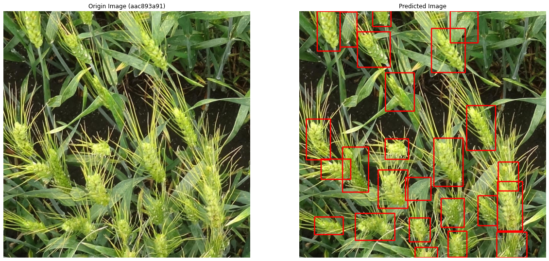
Can you help identify wheat heads using image analysis?

You are attempting to predict bounding boxes around each wheat head in images that have them. If there are no wheat heads, you must predict no bounding boxes.

캐글 주소 : https://www.kaggle.com/c/global-wheat-detection/overview
데이터셋에 대한 논문 : https://arxiv.org/abs/2005.02162


패키지 불러오기

1
2
3
4
5
6
7
8
9
10
11
12
13
14
15
16
17
18
import numpy as np 
import pandas as pd 
import os
from PIL import Image
import cv2
import matplotlib.pyplot as plt

import torch
import torch.nn as nn
from torch.utils.data import Dataset, DataLoader
import torchvision
from torchvision.models.detection.faster_rcnn import FastRCNNPredictor

from sklearn.model_selection import StratifiedKFold
from glob import glob

from albumentations.pytorch.transforms import ToTensorV2
import albumentations as A

하이퍼파라미터 설정

1
2
3
4
5
6
7
args = {
    "TRAIN" : '/kaggle/input/global-wheat-detection/train/',
    "DEVICE" : torch.device('cuda' if torch.cuda.is_available() else 'cpu'),
    "BATCH_SIZE" : 8,
    "NUM_EPOCHS" : 20,
    "NUM_FOLDS" : 5
}

이미지 확인하기

1
2
3
4
img = Image.open('/kaggle/input/global-wheat-detection/train/944c60a15.jpg')

print(img.size)
img.resize((256,256))
1
(1024, 1024)

png

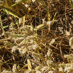
  • 이미지의 크기가 (1024,1024)로 매우 크다.
  • int32, float32 로 이미지 데이터 타입을 바꿔서 메모리 소모량을 최소화하자.
  • float32 보다 float16으로 하면 안되는가
    • 모델 학습 시 gradient update할 때, 소수점 아래 미세한 차이가 결과적으로 큰 차이를 가져온다.
    • float16은 소수점 4번째까지만 저장하게 되고, 그 아래의 값들은 모두 버리게 되어 정보가 손실된다. 모델 성능에까지 영향을 주게 된다.
    • 따라서 이미지의 데이터 타입은 보통 float32으로 설정해준다.
1
print('origin  :', (0.9)**8, '\nfloat16 :', np.float16((0.9)**8), '\nfloat32 :', np.float32((0.9)**8), '\nfloat64 :', np.float64((0.9)**8))
1
2
3
4
origin  : 0.4304672100000001 
float16 : 0.4304 
float32 : 0.43046722 
float64 : 0.4304672100000001

데이터 전처리

  • Detection 대회에서 항상 기억해야할 전처리
    1. 데이터셋 만들기(불러오기)
    2. Data Loader만들기

데이터셋 만들기(불러오기)

  • train 데이터프레임을 보면, bbox의 칼럼값이 str으로 들어가 있다.
  • 각 값을 x, y, w, h칼럼에 각각 넣어주는 처리를 해주자.
  • 아래 코드에서 np.stack() 함수를 이용하면 쉽게 데이터 프레임의 칼럼으로 집어 넣을 수 있다.
  • dtypes을 찍어봐서 x, y, w, h 값들이 숫자형태로 들어갔는지 확인하자.
    • Detection 문제에서 사용할 수 있는 모델(efficientdet, fastrcnn 등)에 따라 bounding box의 전처리가 조금씩 달라질 수 있다.
    • 지금은 fastrcnn모델을 사용할 것이므로 이에 맞는 전처리를 해줘야 한다.
1
2
3
train = pd.read_csv('/kaggle/input/global-wheat-detection/train.csv')
train[['x','y','w','h']] = np.stack(train['bbox'].apply(lambda x : np.fromstring(x[1:-1], sep=',')))
train.head()
image_id width height bbox source x y w h
0 b6ab77fd7 1024 1024 [834.0, 222.0, 56.0, 36.0] usask_1 834.0 222.0 56.0 36.0
1 b6ab77fd7 1024 1024 [226.0, 548.0, 130.0, 58.0] usask_1 226.0 548.0 130.0 58.0
2 b6ab77fd7 1024 1024 [377.0, 504.0, 74.0, 160.0] usask_1 377.0 504.0 74.0 160.0
3 b6ab77fd7 1024 1024 [834.0, 95.0, 109.0, 107.0] usask_1 834.0 95.0 109.0 107.0
4 b6ab77fd7 1024 1024 [26.0, 144.0, 124.0, 117.0] usask_1 26.0 144.0 124.0 117.0
1
train.dtypes
1
2
3
4
5
6
7
8
9
10
image_id     object
width         int64
height        int64
bbox         object
source       object
x           float64
y           float64
w           float64
h           float64
dtype: object

데이터셋 살펴보기

1
print(f"total length : {len(train)}\nunique length : {len(train['image_id'].unique())}")
1
2
total length : 147793
unique length : 3373
  • train셋에서 총 행의 개수가 147793이지만, unique한 개수는 3373개이다. 즉, 한 이미지에 여러 bounding box 값들이 있다는 의미이다.
  • Detection 모델에 데이터를 넣어줄 때 관례적으로 bounding box의 [xmin,ymin, xmax,ymax] 입력받는다.(왼쪽 위, 오른쪽 아래 점)
  • 현재 train 데이터프레임의 bbox 칼럼에서는 [xmin, ymin, width, height]값으로 들어가 있으므로 좌표 역시 전처리 해줘야 한다. 모델 예측한 ouput값은 [xmin,ymin, xmax,ymax]로 나오므로, 역시 제출 시 처리를 해줘야 한다는 것을 까먹지 말자.

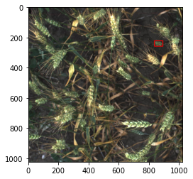
이미지에 Bounding Box 그려보기

1. 이미지에 하나의 bounding box 그려보기

1
2
3
4
5
6
7
8
9
index=0
img = cv2.imread(args["TRAIN"] + train['image_id'][index] + '.jpg', cv2.IMREAD_COLOR)
img = cv2.cvtColor(img, cv2.COLOR_BGR2RGB)
xmin, ymin, w, h = int(train['x'][index]), int(train['y'][index]), int(train['w'][index]), int(train['h'][index])
xmax, ymax = xmin+w, ymin+h

cv2.rectangle(img, (xmin, ymin), (xmax, ymax), (255,0,0), 3)

plt.imshow(img)
1
<matplotlib.image.AxesImage at 0x7f0d019dfc10>

png


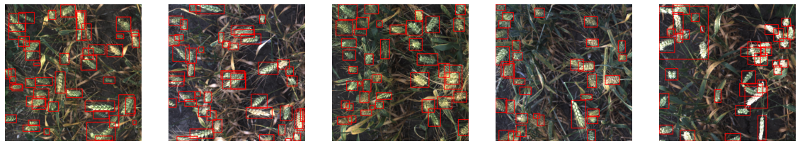
2. 한 이미지에 해당하는 모든 bounding box 그려보기

1
2
3
4
5
6
7
8
9
10
11
12
13
14
15
16
17
18
19
fig, axes = plt.subplots(1, 5)
fig.set_size_inches(20, 15)

for i in range(0,5):
    img_idx = i
    image_id = train['image_id'].unique()[img_idx]
    temp_df = train[train['image_id']==image_id].reset_index()


    img = cv2.imread(f"{args['TRAIN']}{image_id}.jpg", cv2.IMREAD_COLOR)
    img = cv2.cvtColor(img, cv2.COLOR_BGR2RGB)

    for index in range(0,len(temp_df)):
        xmin, ymin, w, h = int(temp_df['x'][index]), int(temp_df['y'][index]), int(temp_df['w'][index]), int(temp_df['h'][index])
        xmax, ymax = xmin+w, ymin+h
        cv2.rectangle(img, (xmin, ymin), (xmax, ymax), (255,0,0), 3)

    axes[i].imshow(img)
    axes[i].axis('off')

png


교차 검증을 위해 Train, Valid 데이터셋 나누기

  • 현재 이미지마다 바운딩박스의 개수가 모두 다르다.
  • 먼저 바운딩박스 개수에 대한 정보를 추가하자. 또한, 현재 데이터에는 source 칼럼에 벼 종류에 대한 정보가 있다. 참고로 벼 종류의 유니크한 개수는 7이다. 이러한 벼 종류 역시 골고루 나눠지게 해야 한다.
  • 바운딩박스의 개수 및 벼 종류에 따라 구간을 나눠서 카테고리를 나눠보자.
  • 예를 들어 0-15개의 바운딩 박스를 갖는 이미지는 a 클래스, 16-30개의 바운딩박스를 갖는 이미지는 b 클래스 …

1. image_id 데이터 가져오기

1
2
df_folds = train[['image_id']].copy()
df_folds
image_id
0 b6ab77fd7
1 b6ab77fd7
2 b6ab77fd7
3 b6ab77fd7
4 b6ab77fd7
... ...
147788 5e0747034
147789 5e0747034
147790 5e0747034
147791 5e0747034
147792 5e0747034

147793 rows × 1 columns


2. image_id 별로 bounding box 개수 count하기

1
2
3
df_folds.loc[:,'bbox_count'] = 1 
df_folds = df_folds.groupby('image_id').count()
df_folds
bbox_count
image_id
00333207f 55
005b0d8bb 20
006a994f7 25
00764ad5d 41
00b5fefed 25
... ...
ffb445410 57
ffbf75e5b 52
ffbfe7cc0 34
ffc870198 41
ffdf83e42 39

3373 rows × 1 columns


3. source 정보 추가하기

1
2
3
4
# 벼(source) 역시 교차검증 나눌 때 클래스별로 나누기
print(f"Unique Number of Source : {train['source'].nunique()}")
df_folds.loc[:, 'source'] = train[['image_id','source']].groupby('image_id').min()["source"]
df_folds
1
Unique Number of Source : 7
bbox_count source
image_id
00333207f 55 arvalis_1
005b0d8bb 20 usask_1
006a994f7 25 inrae_1
00764ad5d 41 inrae_1
00b5fefed 25 arvalis_3
... ... ...
ffb445410 57 rres_1
ffbf75e5b 52 arvalis_1
ffbfe7cc0 34 arvalis_1
ffc870198 41 usask_1
ffdf83e42 39 arvalis_1

3373 rows × 2 columns


4. bbox_count, source 정보를 합친 stratify_group 칼럼 만들기

  • bounding box의 개수의 범위 정보와 source 정보가 담겨져 있는 stratify_group 칼럼 생성한다.
  • stratify_group은 source 종류와 바운딩박스 개수를 15로 나누었을 때의 나머지에 대한 정보가 들어간다.
1
2
3
df_folds.loc[:,'stratify_group'] = np.char.add(df_folds['source'].values.astype(str), 
                                               df_folds['bbox_count'].apply(lambda x : f'_{x//15}').values)
df_folds
bbox_count source stratify_group
image_id
00333207f 55 arvalis_1 arvalis_1_3
005b0d8bb 20 usask_1 usask_1_1
006a994f7 25 inrae_1 inrae_1_1
00764ad5d 41 inrae_1 inrae_1_2
00b5fefed 25 arvalis_3 arvalis_3_1
... ... ... ...
ffb445410 57 rres_1 rres_1_3
ffbf75e5b 52 arvalis_1 arvalis_1_3
ffbfe7cc0 34 arvalis_1 arvalis_1_2
ffc870198 41 usask_1 usask_1_2
ffdf83e42 39 arvalis_1 arvalis_1_2

3373 rows × 3 columns


5. stratify_group의 개수 파악하기

1
2
# bbox 개수 및 source 별 개수
df_folds['stratify_group'].value_counts()
1
2
3
4
5
6
7
8
9
10
11
12
13
14
15
16
17
18
19
20
21
22
23
24
25
26
27
28
29
30
31
32
33
34
35
arvalis_1_2    495
ethz_1_4       364
arvalis_1_3    346
ethz_1_5       214
rres_1_3       172
arvalis_2_1    171
arvalis_3_1    160
arvalis_3_0    154
rres_1_2       145
ethz_1_3       141
inrae_1_1      127
arvalis_1_1    115
arvalis_3_3    104
arvalis_3_2     94
usask_1_1       93
usask_1_2       81
rres_1_4        75
arvalis_1_4     70
arvalis_3_4     40
rres_1_1        39
inrae_1_0       31
arvalis_2_0     26
arvalis_1_5     23
ethz_1_6        18
inrae_1_2       18
usask_1_3       15
usask_1_0       11
ethz_1_2         8
arvalis_3_5      7
arvalis_2_2      7
arvalis_1_6      5
ethz_1_7         2
arvalis_1_0      1
rres_1_5         1
Name: stratify_group, dtype: int64

6. fold 칼럼을 추가하여 데이터 나누기

  • 먼저 fold의 기본값을 0으로 설정하고, StratifiedKFold을 이용하여 stratify_group 기준으로 0~4의 값으로 나눠준다.
1
2
df_folds.loc[:, 'fold']=0
df_folds
bbox_count source stratify_group fold
image_id
00333207f 55 arvalis_1 arvalis_1_3 0
005b0d8bb 20 usask_1 usask_1_1 0
006a994f7 25 inrae_1 inrae_1_1 0
00764ad5d 41 inrae_1 inrae_1_2 0
00b5fefed 25 arvalis_3 arvalis_3_1 0
... ... ... ... ...
ffb445410 57 rres_1 rres_1_3 0
ffbf75e5b 52 arvalis_1 arvalis_1_3 0
ffbfe7cc0 34 arvalis_1 arvalis_1_2 0
ffc870198 41 usask_1 usask_1_2 0
ffdf83e42 39 arvalis_1 arvalis_1_2 0

3373 rows × 4 columns

1
2
3
4
5
6
7
8
9
from sklearn.model_selection import StratifiedKFold

skf = StratifiedKFold(n_splits=5, shuffle=True, random_state=42)

# 그룹 나누기
for i, (train_index, valid_index) in enumerate(skf.split(df_folds,df_folds['stratify_group'])):
    df_folds.loc[df_folds.iloc[valid_index].index,'fold'] = i 
df_folds = df_folds.reset_index()
df_folds
image_id bbox_count source stratify_group fold
0 00333207f 55 arvalis_1 arvalis_1_3 1
1 005b0d8bb 20 usask_1 usask_1_1 3
2 006a994f7 25 inrae_1 inrae_1_1 1
3 00764ad5d 41 inrae_1 inrae_1_2 0
4 00b5fefed 25 arvalis_3 arvalis_3_1 3
... ... ... ... ... ...
3368 ffb445410 57 rres_1 rres_1_3 1
3369 ffbf75e5b 52 arvalis_1 arvalis_1_3 1
3370 ffbfe7cc0 34 arvalis_1 arvalis_1_2 3
3371 ffc870198 41 usask_1 usask_1_2 4
3372 ffdf83e42 39 arvalis_1 arvalis_1_2 4

3373 rows × 5 columns


7. fold별로 stratify_group의 개수 파악하기

  • fold 별로 잘 나누어졌는지 확인한다.
1
2
3
4
for i in range(5):
    print("*"*30,'\n')
    print(f"FOLD : {i}\n")
    print(df_folds[df_folds["fold"]==i]['stratify_group'].value_counts(),'\n')
1
2
3
4
5
6
7
8
9
10
11
12
13
14
15
16
17
18
19
20
21
22
23
24
25
26
27
28
29
30
31
32
33
34
35
36
37
38
39
40
41
42
43
44
45
46
47
48
49
50
51
52
53
54
55
56
57
58
59
60
61
62
63
64
65
66
67
68
69
70
71
72
73
74
75
76
77
78
79
80
81
82
83
84
85
86
87
88
89
90
91
92
93
94
95
96
97
98
99
100
101
102
103
104
105
106
107
108
109
110
111
112
113
114
115
116
117
118
119
120
121
122
123
124
125
126
127
128
129
130
131
132
133
134
135
136
137
138
139
140
141
142
143
144
145
146
147
148
149
150
151
152
153
154
155
156
157
158
159
160
161
162
163
164
165
166
167
168
169
170
171
172
173
174
175
176
177
178
179
180
181
182
183
184
185
186
187
188
****************************** 

FOLD : 0

arvalis_1_2    99
ethz_1_4       72
arvalis_1_3    70
ethz_1_5       43
rres_1_3       35
arvalis_2_1    34
arvalis_3_1    32
arvalis_3_0    31
rres_1_2       29
ethz_1_3       28
inrae_1_1      26
arvalis_1_1    23
arvalis_3_3    21
usask_1_1      18
arvalis_3_2    18
usask_1_2      16
rres_1_4       15
arvalis_1_4    14
arvalis_3_4     8
rres_1_1        8
inrae_1_0       7
arvalis_2_0     6
ethz_1_6        4
arvalis_1_5     4
inrae_1_2       3
usask_1_3       3
usask_1_0       2
ethz_1_2        2
arvalis_3_5     1
arvalis_1_0     1
arvalis_1_6     1
arvalis_2_2     1
Name: stratify_group, dtype: int64 

****************************** 

FOLD : 1

arvalis_1_2    99
ethz_1_4       73
arvalis_1_3    69
ethz_1_5       43
arvalis_2_1    35
rres_1_3       34
arvalis_3_1    32
arvalis_3_0    31
rres_1_2       29
ethz_1_3       28
inrae_1_1      25
arvalis_1_1    23
arvalis_3_3    20
usask_1_1      19
arvalis_3_2    19
usask_1_2      16
rres_1_4       15
arvalis_1_4    14
arvalis_3_4     8
rres_1_1        8
inrae_1_0       6
arvalis_2_0     5
arvalis_1_5     5
ethz_1_6        4
inrae_1_2       4
usask_1_3       3
usask_1_0       2
arvalis_3_5     2
ethz_1_2        1
arvalis_1_6     1
arvalis_2_2     1
rres_1_5        1
Name: stratify_group, dtype: int64 

****************************** 

FOLD : 2

arvalis_1_2    99
ethz_1_4       73
arvalis_1_3    69
ethz_1_5       42
rres_1_3       34
arvalis_2_1    34
arvalis_3_1    32
arvalis_3_0    31
rres_1_2       29
ethz_1_3       28
inrae_1_1      25
arvalis_1_1    23
arvalis_3_3    21
usask_1_1      19
arvalis_3_2    19
usask_1_2      16
rres_1_4       15
arvalis_1_4    14
arvalis_3_4     8
rres_1_1        8
inrae_1_0       6
arvalis_2_0     5
arvalis_1_5     5
ethz_1_6        4
inrae_1_2       4
usask_1_0       3
usask_1_3       3
arvalis_3_5     2
arvalis_2_2     2
ethz_1_2        1
arvalis_1_6     1
Name: stratify_group, dtype: int64 

****************************** 

FOLD : 3

arvalis_1_2    99
ethz_1_4       73
arvalis_1_3    69
ethz_1_5       43
rres_1_3       34
arvalis_2_1    34
arvalis_3_1    32
arvalis_3_0    30
rres_1_2       29
ethz_1_3       28
inrae_1_1      25
arvalis_1_1    23
arvalis_3_3    21
usask_1_1      19
arvalis_3_2    19
usask_1_2      17
rres_1_4       15
arvalis_1_4    14
arvalis_3_4     8
rres_1_1        7
inrae_1_0       6
arvalis_2_0     5
arvalis_1_5     5
inrae_1_2       4
ethz_1_6        3
usask_1_3       3
arvalis_2_2     2
usask_1_0       2
ethz_1_2        2
arvalis_3_5     1
arvalis_1_6     1
ethz_1_7        1
Name: stratify_group, dtype: int64 

****************************** 

FOLD : 4

arvalis_1_2    99
ethz_1_4       73
arvalis_1_3    69
ethz_1_5       43
rres_1_3       35
arvalis_2_1    34
arvalis_3_1    32
arvalis_3_0    31
rres_1_2       29
ethz_1_3       29
inrae_1_1      26
arvalis_1_1    23
arvalis_3_3    21
arvalis_3_2    19
usask_1_1      18
usask_1_2      16
rres_1_4       15
arvalis_1_4    14
arvalis_3_4     8
rres_1_1        8
inrae_1_0       6
arvalis_2_0     5
arvalis_1_5     4
ethz_1_6        3
usask_1_3       3
inrae_1_2       3
usask_1_0       2
ethz_1_2        2
arvalis_3_5     1
ethz_1_7        1
arvalis_1_6     1
arvalis_2_2     1
Name: stratify_group, dtype: int64 

데이터 로더 만들기

1
2
3
4
5
6
7
8
9
10
11
12
13
14
15
16
17
18
19
20
21
22
23
24
25
26
27
28
29
30
31
32
33
34
35
36
37
38
39
40
41
42
43
44
45
46
47
48
49
class WheatDataset(Dataset):
    def __init__(self, dataframe, image_dir, transforms=None):
        super().__init__()
        self.df = dataframe
        self.image_dir = image_dir
        self.transforms = transforms
        self.image_ids = dataframe['image_id'].unique()
        
    def __getitem__(self, index):
        image_id = self.image_ids[index]
        
        # bounding box
        records = self.df[self.df['image_id'] == image_id]
        boxes = records[['x', 'y', 'w', 'h']].values # values -> dataframe to array
        
        # w,h to xmax, ymax
        boxes[:,2] = boxes[:,2] + boxes[:,0]
        boxes[:,3] = boxes[:,3] + boxes[:,1]
        
        # label
        # 다중 분류가 아니기 때문에(wheat or background), 모델 학습이 돌아갈 수 있게끔 모양만 만들어 두자.
        # 한 이미지에 대한 모든 bounding box의 개수를 가져온다.
        labels = torch.ones(len(records), dtype = torch.int64)
        
        # image
        img = cv2.imread(self.image_dir + image_id + '.jpg', cv2.IMREAD_COLOR)
        img = cv2.cvtColor(img, cv2.COLOR_BGR2RGB).astype(np.float32)
        img = img / 255.0
        
        # 데이터를 dictionary 형태로 보관하자.
        # faster rcnn model에 들어갈 때, target의 key값들은 아래와 일치하도록 해야 한다. 안그러면 KeyError 발생한다.
        target = {'labels' : labels, 'boxes' : boxes}
        
        # transforms
        # img 뿐만 아니라 bounding box, label 모두 tensor 형태로 바꿔야 한다.
        if self.transforms:
            # image, bboxes라는 key값 자체가 있기 때문에 반드시 이름을 이와 같게 해야 한다.
            sample = {'image' : img, 'bboxes' : boxes, 'labels' : labels}
            
            sample = self.transforms(**sample)
            img = sample['image']
            
            target['boxes'] = torch.stack(tuple(map(torch.tensor, zip(sample['bboxes'])))).squeeze(1)
        
        return img, target, image_id

        
    def __len__(self):
        return len(self.image_ids)

Bounding Box를 Tensor로 만들 때 주의해야할 점

  • 데이터로더의 __getitem__의 마지막 부분을 보면, boxes값들을 tensor로 만들어주는 코드가 있다.
  • 밑의 예시를 보며 각각의 코드들이 어떤 역할을 하는지 이해할 필요가 있다.
1
2
x = {'boxes' : [[1,2,3], [4,5,6], [7,8,9]]}
x['boxes']
1
[[1, 2, 3], [4, 5, 6], [7, 8, 9]]

1
print(f"Using unpacking operator : {list(zip(*x['boxes']))}\nNot using unpacking operator : {list(zip(x['boxes']))}")
1
2
Using unpacking operator : [(1, 4, 7), (2, 5, 8), (3, 6, 9)]
Not using unpacking operator : [([1, 2, 3],), ([4, 5, 6],), ([7, 8, 9],)]
  • unpacking operator를 사용하면 값들의 순서가 바뀐 것을 볼 수 있다. 이렇게 바뀐 순서를 다시 원래대로 돌려주기 위해 permute함수가 사용된 것이다.

1
2
using_permute = torch.stack(tuple(map(torch.tensor, zip(*x['boxes'])))).permute(1,0)
print(f"Using permute : \n{using_permute}\nShape : {using_permute.shape}")
1
2
3
4
5
Using permute : 
tensor([[1, 2, 3],
        [4, 5, 6],
        [7, 8, 9]])
Shape : torch.Size([3, 3])

  • 코드를 더 간단하게 만들기 위해 squeeze를 사용해도 괜찮다.
1
2
using_squeeze = torch.stack(tuple(map(torch.tensor, zip(x['boxes'])))).squeeze(1)
print(f'Using squeeze : \n{using_squeeze}\nShape : {using_squeeze.shape}')
1
2
3
4
5
Using squeeze : 
tensor([[1, 2, 3],
        [4, 5, 6],
        [7, 8, 9]])
Shape : torch.Size([3, 3])

transforms 함수 만들기

1
2
3
4
5
6
7
8
9
10
11
12
def get_train_transform():
    return A.Compose([
        A.Flip(0.5),
        ToTensorV2()
    ], bbox_params = A.BboxParams(format = 'pascal_voc', label_fields = ['labels'])
    )

def get_valid_transform():
    return A.Compose([
        ToTensorV2()
    ], bbox_params = A.BboxParams(format = 'pascal_voc', label_fields = ['labels'])
    )

"Stack" 관련 에러 날 경우

RuntimeError: stack expects each tensor to be equal size, but got [49, 4] at entry 0 and [26, 4] at entry 1

  • 이러한 에러가 날 시, DataLoader 설정 시 collate_fn 옵션을 넣어줘야 한다.
  • 특정 상황에서 batch별로 데이터가 잘 안묶여서 생기는 에러이므로, 이러한 오류가 나면 아래와 같은 함수를 설정하여 옵션에 넣어주자.
1
2
def collate_fn(batch):
    return tuple(zip(*batch))
1
2
train_dataset = WheatDataset(train, args["TRAIN"], transforms = get_train_transform())
train_loader = DataLoader(train_dataset, batch_size = args["BATCH_SIZE"], shuffle = True, collate_fn = collate_fn, num_workers = 4)

학습하기

모델 불러오기

  • 모델은 fasterrcnn_resnet50_fpn을 사용한다.
    • fpn : feature pyramid network로, 기존 모델 구조에서 보다 발전된 형태이다. 참고 : https://eehoeskrap.tistory.com/300
    • Backbone은 resnet50을 사용한다.
  • 모델의 구조를 보면, Dropout, BatchNormalization 등의 레이어 층을 볼 수 있다.
    • Dropout : 모델이 train 데이터셋을 통해 중요한 노드(요소)들을 집중적으로 학습하다 보니, test셋과 같은 새로운 데이터가 왔을 때 예측을 잘 하지 못하는 경우가 발생한다. train셋에 과적합 되었기 때문이다. 이를 개선하기 위해 Dropout옵션을 정해주는 것이다. 또한 매번 다른 노드들로 학습을 하다 보니, 앙상블의 효과도 얻을 수 있다.
      • 만약 Dropout(0.3)이면, 0.3만큼의 임의의 노드를 사용하지 않는다는 의미이다.
      • 이 때 0이 되지 않은 0.7에 해당하는 값은 (1/0.7) 만큼 scale이 된다. 따라서 (1/0.7 = 1.4286…)이 되는 것이다.
    • BatchNorm : 배치로 들어오는 데이터에 규제를 넣어주는 것이다. 학습 속도 및 학습 성능에 영향을 준다.
    • 참고 블로그 : https://gaussian37.github.io/dl-pytorch-snippets/
1
2
model = torchvision.models.detection.fasterrcnn_resnet50_fpn(pretrained=True)
model
1
2
3
4
5
6
7
8
9
10
11
12
13
14
15
16
17
18
19
20
21
22
23
24
1
2
3
4
5
6
7
8
9
10
11
12
13
14
15
16
17
18
19
20
21
22
23
24
FasterRCNN(
  (transform): GeneralizedRCNNTransform(
      Normalize(mean=[0.485, 0.456, 0.406], std=[0.229, 0.224, 0.225])
      Resize(min_size=(800,), max_size=1333, mode='bilinear')
  )
  (backbone): BackboneWithFPN(
    (body): IntermediateLayerGetter(
      (conv1): Conv2d(3, 64, kernel_size=(7, 7), stride=(2, 2), padding=(3, 3), bias=False)
      (bn1): FrozenBatchNorm2d(64)
      (relu): ReLU(inplace=True)
      (maxpool): MaxPool2d(kernel_size=3, stride=2, padding=1, dilation=1, ceil_mode=False)
      (layer1): Sequential(
        (0): Bottleneck(
          (conv1): Conv2d(64, 64, kernel_size=(1, 1), stride=(1, 1), bias=False)
          (bn1): FrozenBatchNorm2d(64)
          (conv2): Conv2d(64, 64, kernel_size=(3, 3), stride=(1, 1), padding=(1, 1), bias=False)
          (bn2): FrozenBatchNorm2d(64)
          (conv3): Conv2d(64, 256, kernel_size=(1, 1), stride=(1, 1), bias=False)
          (bn3): FrozenBatchNorm2d(256)
          (relu): ReLU(inplace=True)
          (downsample): Sequential(
            (0): Conv2d(64, 256, kernel_size=(1, 1), stride=(1, 1), bias=False)
            (1): FrozenBatchNorm2d(256)
          )


.
.
.

1
2
3
4
5
6
7
8
9
10
11
12
13
14
15
16
17
18
19
20
21
22
23
24
25
26
27
28
29
30
31
32
33
34
35
36
        (fpn): FeaturePyramidNetwork(
          (inner_blocks): ModuleList(
            (0): Conv2d(256, 256, kernel_size=(1, 1), stride=(1, 1))
            (1): Conv2d(512, 256, kernel_size=(1, 1), stride=(1, 1))
            (2): Conv2d(1024, 256, kernel_size=(1, 1), stride=(1, 1))
            (3): Conv2d(2048, 256, kernel_size=(1, 1), stride=(1, 1))
          )
          (layer_blocks): ModuleList(
            (0): Conv2d(256, 256, kernel_size=(3, 3), stride=(1, 1), padding=(1, 1))
            (1): Conv2d(256, 256, kernel_size=(3, 3), stride=(1, 1), padding=(1, 1))
            (2): Conv2d(256, 256, kernel_size=(3, 3), stride=(1, 1), padding=(1, 1))
            (3): Conv2d(256, 256, kernel_size=(3, 3), stride=(1, 1), padding=(1, 1))
          )
          (extra_blocks): LastLevelMaxPool()
        )
      )
      (rpn): RegionProposalNetwork(
        (anchor_generator): AnchorGenerator()
        (head): RPNHead(
          (conv): Conv2d(256, 256, kernel_size=(3, 3), stride=(1, 1), padding=(1, 1))
          (cls_logits): Conv2d(256, 3, kernel_size=(1, 1), stride=(1, 1))
          (bbox_pred): Conv2d(256, 12, kernel_size=(1, 1), stride=(1, 1))
        )
      )
      (roi_heads): RoIHeads(
        (box_roi_pool): MultiScaleRoIAlign()
        (box_head): TwoMLPHead(
          (fc6): Linear(in_features=12544, out_features=1024, bias=True)
          (fc7): Linear(in_features=1024, out_features=1024, bias=True)
        )
        (box_predictor): FastRCNNPredictor(
          (cls_score): Linear(in_features=1024, out_features=91, bias=True)
          (bbox_pred): Linear(in_features=1024, out_features=364, bias=True)
        )
      )
    )

모델 out_features 바꿔주기

  • 모델 구조를 보면, 마지막 box_predictor를 보면 cls_scoreout_features가 91이다.
  • 현재 우리는 wheat / background 라는 두 개의 class를 분류하는 문제를 갖고 있으므로, out_features=2로 바꿔줘야 한다.
  • bbox_pred 역시 class 개수에 따라 바꿔준다. 로 자동적으로 바뀐다.
    • torch.nn.Linear로 바꿀 시, cls_score, bbox_pred 모두 바꿔줘야 하고, torchvision.models.detection.faster_rcnn.FastRCNNPredictor로 접근하여 바꿀 시, bbox_predcls_score*4 로 자동적으로 바뀐다.

방법 1

1
2
3
model.roi_heads.box_predictor = FastRCNNPredictor(1024,2)

model.roi_heads.box_predictor
1
2
3
4
1
2
3
4
FastRCNNPredictor(
  (cls_score): Linear(in_features=1024, out_features=2, bias=True)
  (bbox_pred): Linear(in_features=1024, out_features=8, bias=True)
)

방법 2

1
2
3
4
model.roi_heads.box_predictor.cls_score = nn.Linear(in_features=1024, out_features=2, bias=True)
model.roi_heads.box_predictor.bbox_pred = nn.Linear(in_features=1024, out_features=8, bias=True)

model.roi_heads.box_predictor
1
2
3
4
1
2
3
4
FastRCNNPredictor(
  (cls_score): Linear(in_features=1024, out_features=2, bias=True)
  (bbox_pred): Linear(in_features=1024, out_features=8, bias=True)
)

1
2
# model to GPU
model.to(args["DEVICE"])
1
2
3
4
5
6
7
8
9
10
11
12
13
14
15
16
17
18
19
20
21
22
23
24
1
2
3
4
5
6
7
8
9
10
11
12
13
14
15
16
17
18
19
20
21
22
23
24
FasterRCNN(
  (transform): GeneralizedRCNNTransform(
      Normalize(mean=[0.485, 0.456, 0.406], std=[0.229, 0.224, 0.225])
      Resize(min_size=(800,), max_size=1333, mode='bilinear')
  )
  (backbone): BackboneWithFPN(
    (body): IntermediateLayerGetter(
      (conv1): Conv2d(3, 64, kernel_size=(7, 7), stride=(2, 2), padding=(3, 3), bias=False)
      (bn1): FrozenBatchNorm2d(64)
      (relu): ReLU(inplace=True)
      (maxpool): MaxPool2d(kernel_size=3, stride=2, padding=1, dilation=1, ceil_mode=False)
      (layer1): Sequential(
        (0): Bottleneck(
          (conv1): Conv2d(64, 64, kernel_size=(1, 1), stride=(1, 1), bias=False)
          (bn1): FrozenBatchNorm2d(64)
          (conv2): Conv2d(64, 64, kernel_size=(3, 3), stride=(1, 1), padding=(1, 1), bias=False)
          (bn2): FrozenBatchNorm2d(64)
          (conv3): Conv2d(64, 256, kernel_size=(1, 1), stride=(1, 1), bias=False)
          (bn3): FrozenBatchNorm2d(256)
          (relu): ReLU(inplace=True)
          (downsample): Sequential(
            (0): Conv2d(64, 256, kernel_size=(1, 1), stride=(1, 1), bias=False)
            (1): FrozenBatchNorm2d(256)
          )


.
.
.

1
2
3
4
5
6
7
8
9
10
11
12
13
14
15
16
17
18
19
20
21
22
23
24
25
26
27
28
29
30
31
32
33
34
35
36
        (fpn): FeaturePyramidNetwork(
          (inner_blocks): ModuleList(
            (0): Conv2d(256, 256, kernel_size=(1, 1), stride=(1, 1))
            (1): Conv2d(512, 256, kernel_size=(1, 1), stride=(1, 1))
            (2): Conv2d(1024, 256, kernel_size=(1, 1), stride=(1, 1))
            (3): Conv2d(2048, 256, kernel_size=(1, 1), stride=(1, 1))
          )
          (layer_blocks): ModuleList(
            (0): Conv2d(256, 256, kernel_size=(3, 3), stride=(1, 1), padding=(1, 1))
            (1): Conv2d(256, 256, kernel_size=(3, 3), stride=(1, 1), padding=(1, 1))
            (2): Conv2d(256, 256, kernel_size=(3, 3), stride=(1, 1), padding=(1, 1))
            (3): Conv2d(256, 256, kernel_size=(3, 3), stride=(1, 1), padding=(1, 1))
          )
          (extra_blocks): LastLevelMaxPool()
        )
      )
      (rpn): RegionProposalNetwork(
        (anchor_generator): AnchorGenerator()
        (head): RPNHead(
          (conv): Conv2d(256, 256, kernel_size=(3, 3), stride=(1, 1), padding=(1, 1))
          (cls_logits): Conv2d(256, 3, kernel_size=(1, 1), stride=(1, 1))
          (bbox_pred): Conv2d(256, 12, kernel_size=(1, 1), stride=(1, 1))
        )
      )
      (roi_heads): RoIHeads(
        (box_roi_pool): MultiScaleRoIAlign()
        (box_head): TwoMLPHead(
          (fc6): Linear(in_features=12544, out_features=1024, bias=True)
          (fc7): Linear(in_features=1024, out_features=1024, bias=True)
        )
        (box_predictor): FastRCNNPredictor(
          (cls_score): Linear(in_features=1024, out_features=2, bias=True)
          (bbox_pred): Linear(in_features=1024, out_features=8, bias=True)
        )
      )
    )

업데이트할 Parameters 설정

  • model의 parameters 중, requires_grad=True, 즉 freeze가 안된 파라미터들을 가져와서 학습하겠다는 의미이다.
  • Epoch를 돌며 경사하강법으로 학습할 파라미터이다.
1
2
params = [x for x in model.parameters() if x.requires_grad]
params[-5:]
1
2
3
4
5
6
7
8
9
10
11
12
13
14
15
16
17
18
19
20
21
22
23
24
25
26
27
[Parameter containing:
 tensor([ 0.0086,  0.0309,  0.0581,  ..., -0.0181,  0.0325,  0.0189],
        device='cuda:0', requires_grad=True),
 Parameter containing:
 tensor([[-7.6312e-03,  2.0107e-02,  1.4423e-02,  ...,  6.0976e-05,
           3.0176e-02,  2.4542e-02],
         [ 1.1975e-02,  3.7853e-03,  1.3403e-02,  ..., -2.7104e-02,
          -2.0492e-02, -1.9000e-02]], device='cuda:0', requires_grad=True),
 Parameter containing:
 tensor([0.0195, 0.0138], device='cuda:0', requires_grad=True),
 Parameter containing:
 tensor([[-1.7756e-02,  1.4171e-03,  1.5141e-02,  ...,  2.7508e-02,
          -1.1840e-02, -1.3901e-02],
         [-1.7905e-02, -1.7732e-02, -1.7152e-02,  ...,  7.7827e-03,
           1.2814e-02, -1.0298e-02],
         [-2.6198e-02,  2.3477e-05, -2.5067e-03,  ..., -2.8354e-02,
          -6.5023e-03,  1.1452e-02],
         ...,
         [-2.0409e-02,  1.9236e-02,  6.2685e-03,  ...,  2.4985e-02,
          -2.8892e-02, -2.0194e-03],
         [-5.7999e-03, -1.4193e-02,  8.6269e-03,  ..., -2.1297e-02,
           1.7533e-03, -1.9947e-02],
         [-2.9891e-03, -2.0081e-02,  2.4276e-03,  ...,  1.5759e-02,
          -1.5163e-02,  2.7659e-02]], device='cuda:0', requires_grad=True),
 Parameter containing:
 tensor([-0.0081,  0.0307,  0.0157, -0.0003, -0.0152, -0.0005,  0.0208, -0.0266],
        device='cuda:0', requires_grad=True)]

Optimizer 설정

  • AdamW 등 Detection 문제에서 평균적으로 더 좋은 성능을 보이는 옵티마이저가 있지만, 지금은 Adam을 사용해보자.
1
optimizer = torch.optim.Adam(params = params, lr=0.001)

Averager 클래스 설정

  • Averager는 loss 값을 계산할 때 사용한다.
  • Faster Rcnn 모델에서 내부적으로 손실값을 계산할때 사용하는 class로, 이미 구현이 되어있다.
  • 모델마다 이러한 Averager들이 조금씩 다를 수 있으므로, 다른 모델을 사용할 때 검색해서 한번 찾아보자.
1
2
3
4
5
6
7
8
9
10
11
12
13
14
15
16
17
18
19
20
21
class Averager:
    def __init__(self):
        self.current_total = 0.0
        self.iterations = 0.0

    def send(self, value):
        self.current_total += value
        self.iterations += 1

    @property
    def value(self):
        if self.iterations == 0:
            return 0
        else:
            return 1.0 * self.current_total / self.iterations # 평균값

    def reset(self): # 초기화
        self.current_total = 0.0
        self.iterations = 0.0
        
loss_hist = Averager() 

Validation 함수

  • pytorch의 faster-rcnn 모델을 사용할 시, model.eval()은 loss가 아닌 예측 바운딩박스 좌표값들을 돌려준다. 우선은 with torch.no_grad()만 적용하여 validation loss를 계산해보자.

참고 : https://stackoverflow.com/questions/60339336/validation-loss-for-pytorch-faster-rcnn

1
2
3
4
5
6
7
8
9
10
11
12
13
14
15
# validation function
def validation(model, valid_loader, args):
    valid_loss = 0

    for images, targets, image_ids in valid_loader:
        if torch.cuda.is_available():
            images = list(x.to(args["DEVICE"]) for x in images)
            targets = [{k:v.to(args["DEVICE"]) for k,v in t.items()} for t in targets]

        val_loss_dict = model(images, targets)
        val_losses = sum(x for x in val_loss_dict.values())
        valid_loss += val_losses.item()


    return valid_loss / len(valid_loader)

모델 학습하기

  • 모델은 5번의 교차검증으로 훈련한다.

단일 모델 훈련 코드

1
2
3
4
5
6
7
8
9
10
11
12
13
14
15
16
17
18
19
20
21
22
23
24
25
26
27
28
29
30
31
32
33
34
35
36
37
38
39
40
41
42
43
44
45
46
47
48
49
50
51
52
53
def train_model(model, train_loader, valid_loader, optimizer, args):
    steps = 0
    total_step = len(train_loader)
    iterations = 1

    for epoch in range(args["NUM_EPOCHS"]):

        loss_hist.reset()

        for images, targets, image_ids in train_loader:

            # Data to GPU
            images = list(x.to(args["DEVICE"]) for x in images)
            targets = [{k:v.to(args["DEVICE"]) for k,v in t.items()} for t in targets]
            steps += 1

            # Label classification, BoundingBox Regression의 Loss 값이 Ditcionary 형태로 나온다.
            loss_dict = model(images, targets)

            # Dict 형태의 loss_dict에서 .values()로 key:values에서 values를 가져온다.
            losses = sum(x for x in loss_dict.values())

            # losses를 print해보면 tensor()로 감싸져 있다. .item()으로 숫자만 가져오자.
            loss_value = losses.item()

            # loss_hist에 loss_value를 저장한다.
            loss_hist.send(loss_value)

            # optimizer 업데이트 시 항상 나오는 삼총사

            # 1. 기울기 0으로 초기화
            optimizer.zero_grad()
            # 2. 역전파
            losses.backward()
            # 3. 업데이트
            optimizer.step()

            # 10번마다 loss값 출력
            if iterations % 100 == 0:
                print(f"{iterations} iterations ... Loss : {loss_value}")

            iterations +=1
            
            if steps % total_step == 0:
                with torch.no_grad():
                    valid_loss = validation(model, valid_loader, args) 
                
                print("Epoch: {}/{}.. ".format(epoch+1,args['NUM_EPOCHS']),
                     "Training Loss: {:.6f}..".format(loss_hist.value),
                     "Valid Loss: {:.6f}..".format(valid_loss))
                
                step = 0
    return

교차검증 훈련

  • 5번의 교차 검증을 진행한다. 아래 출력창을 보면 로스값이 떨어지는 것을 확인할 수 있다.
1
train_fold = pd.merge(train, df_folds, on='image_id', how='left')
1
2
3
4
5
6
7
8
9
10
11
12
13
14
15
16
17
18
19
20
21
22
23
24
25
26
27
28
29
30
31
32
33
def train_folds(dataframe, args):
    for fold in range(args["NUM_FOLDS"]):

        # Model & Optimizer
        model = torchvision.models.detection.fasterrcnn_resnet50_fpn(pretrained=True)
        model.roi_heads.box_predictor.cls_score = nn.Linear(in_features=1024, out_features=2, bias=True)
        model.roi_heads.box_predictor.bbox_pred = nn.Linear(in_features=1024, out_features=8, bias=True)
        model.to(args["DEVICE"])
        params = [x for x in model.parameters() if x.requires_grad]
        optimizer = torch.optim.Adam(params = params, lr=0.001)

        train_ = train_fold[train_fold["fold"]!=fold].reset_index(drop=True)
        valid_ = train_fold[train_fold["fold"]==fold].reset_index(drop=True)

        # Train Loader & Valid Loader
        train_dataset = WheatDataset(train_, args["TRAIN"], transforms = get_train_transform())
        train_loader = DataLoader(train_dataset,
                                  batch_size = args["BATCH_SIZE"], 
                                  shuffle = True,
                                  collate_fn = collate_fn,
                                  num_workers = 4)
        valid_dataset = WheatDataset(valid_, args["TRAIN"], transforms = get_valid_transform())
        valid_loader = DataLoader(valid_dataset,
                                  batch_size = 1, 
                                  shuffle = False,
                                  collate_fn = collate_fn,
                                  num_workers = 4)

        print(f"\n{fold+1}/{args['NUM_FOLDS']} Cross Validation Training Starts ...\n")
        train_model(model, train_loader, valid_loader, optimizer, args)
        print(f"\n{fold+1}/{args['NUM_FOLDS']} Cross Validation Training Ends ...\n")
        torch.save(model.state_dict(), f"fold{fold}_model.pth")
    return
1
train_folds(train_fold, args)
1
2
3
4
5
6
7
8
9
10
11
12
13
14
15
16
17
18
19
20
21
22
1/5 Cross Validation Training Starts ...

100 iterations ... Loss : 1.7992744816770365
200 iterations ... Loss : 1.3215401355936756
300 iterations ... Loss : 1.2728456529162266
Epoch: 1/20..  Training Loss: 1.705802.. Valid Loss: 1.148290..
400 iterations ... Loss : 1.1416268536681002
500 iterations ... Loss : 0.9909895147586031
600 iterations ... Loss : 1.0571585424735501
Epoch: 2/20..  Training Loss: 1.031144.. Valid Loss: 1.045934..
700 iterations ... Loss : 1.0805089997351918
800 iterations ... Loss : 0.9486090712623582
900 iterations ... Loss : 0.8159377695012606
1000 iterations ... Loss : 0.9475474243279667
Epoch: 3/20..  Training Loss: 0.931789.. Valid Loss: 0.931303..
1100 iterations ... Loss : 0.903436008694743
1200 iterations ... Loss : 0.8769005698768707
1300 iterations ... Loss : 0.7356736096027937
Epoch: 4/20..  Training Loss: 0.882577.. Valid Loss: 0.892810..
1400 iterations ... Loss : 0.841289657854777
1500 iterations ... Loss : 0.828545476986028
1600 iterations ... Loss : 0.8009961004305629

모델 저장하기

  • 모델을 저장하는 방법은 여러 가지이다.
      1. 모든 epoch마다 모델을 저정하는 방법
      1. EarlyStopping을 사용하여 최소 loss 값을 보이는 모델만 저장하는 방법
  • 사용할 방법을 코드로 구현해서 적용하면 된다.

마무리

  • Object Detection - 이진 분류 대회에 대한 기본적인 Base line 코드를 공부해봤다.
  • 교차검증을 위해 Train, Valid 셋을 나눌 때, stratify_group을 만들었는데, 이는 최대한 데이터 분포를 고르게 하여 특정 fold에서 모델이 과적합 되지 않게 하기 위함이었다.
  • 모델 성능을 더 높이기 위한 여러 방법들을(하이퍼 파라미터 조정, 데이터 전처리, 모델 바꿔서 학습해보기 등) 더 공부해보고 적용해보자.
  • 저장한 모델로 test 셋 예측 및 제출하기까지의 방법은 Weighted Boxes Fusion 글을 참고하면 된다.

  • Test데이터 추론에는 Pre-trained faster-rcnn 모델을 5번의 교차검증으로 훈련한 후, weighted boxes fusion방법을 적용했다.
  • 리더보드 점수는 private : 0.5870, public : 0.6735
    • 참고 : 리더보드상 1위 private : 0.6897, 1위 public : 0.7746

참고 자료

0%