Blindness Classification

대회 소개

png

안저 이미지를 통한 Diabetic retinopathy(DR, 당뇨성 망막증) 악화 정도 분류 대회
모델 구조에 SEBlock을 추가하여 모델 복잡도를 크게 증가시키지 않으면서 성능을 향상시킬 수 있습니다.

APTOS 2019 Blindness Detection

Detect diabetic retinopathy to stop blindness before it’s too late
https://www.kaggle.com/c/aptos2019-blindness-detection

평가 지표 : Quadratic weighted kappa


요약

이번 프로젝트는 안저 이미지 데이터를 사용하여 당뇨성 망막증의 증상을 분류하는 모델을 구현하는 것입니다. 당뇨성 망막증은 당뇨병에 의해 망막의 미세혈관이 손상되어 발생하는 질병입니다. 세계 각국의 실명 원인 중에서 높은 비중을 차지하고 있기에 이를 초기에 발견하고 치료하는 것이 중요합니다. 하지만 충분한 의료 인력 및 인프라가 갖추어지지 않은 환경에서 이러한 질병을 발견하고 예방하기란 쉽지 않은 상황입니다. 이 대회에서는 당뇨성 망막증을 식별해내는 인공지능 모델을 개발하여 어떤 환경에서도 망막병증 환자들을 쉽고 빠르게 파악할 수 있기를 기대하고 있습니다.

데이터는 kaggle에서 진행된 APTOS 2019 Blindness Detection에서 제공하는 안저 이미지들입니다. 전체 이미지의 개수는 3662개이고, 각각 0~4 까지의 정수로 레이블링이 되어있습니다. 숫자가 높을수록 병증이 악화됨을 의미합니다. 대회의 평가 지표는 Quadratic weighted kappa입니다. 실제 레이블에서 모델의 예측값이 멀어질수록 더 큰 loss를 주는 방식이기 때문에, 이러한 레이블별 거리를 고려할 수 있도록 모델 학습시 crossentropy loss 대신 mean squared error를 사용했습니다.

모델은 Pre-trained된 ResNet18을 사용했으며, 모델 구조에 Squeeze and Excitation block을 추가했습니다. SE block는 feature map의 정보를 요약하고 그 중요도에 따라 채널 단위로 새로운 가중치를 주는 방식으로, 일종의 attention mechanism이라고 볼 수 있습니다. 이 방식을 제안한 [4]의 저자들은 SE block가 모델 구조 어떤 곳이라도 바로 붙일 수 있고, 계산 복잡도를 크게 증가시키지 않으면서도 모델의 성능을 많이 높일 수 있다는 장점이 있다고 말합니다.

아래는 앞서 이 프로젝트에서 적용했던 방식들을 비교한 표입니다. 모두 동일한 전처리(trim and resize(150,150)), 하이퍼 파라미터(learning rate=0.001, weight decay=0.005) 및 early stopping(patient=10) 조건을 사용했습니다. MSE loss를 사용했을 때 crossentropy loss보다 Test셋과 Valid셋 모두에서 더 높은 성능을 보여주었습니다(파란색). 또한 동일하게 MSE loss를 사용하는 상황에서는 SE block을 추가한 경우 Test 셋에 대해서는 private, public score 모두 향상되었고, 학습시에는 더 낮은 valid loss를 보여주었습니다(빨간색).

Model Loss Private Score Public Score Valid QWK Valid Loss
ResNet18 CrossEntropy 0.7183 0.4173 0.8142 0.6464
ResNet18 MSE 0.7610 0.5091 0.8599 0.4247
ResNet18 + SEBlock MSE 0.8310 0.6766 0.8491 0.4059

이번 프로젝트에서는 기본적인 전처리를 적용한 baseline 모델을 구현했습니다. 이후 정교한 하이퍼파라미터 튜닝이나 이미지 resize 및 여러 augmentation을 적용하여 모델의 성능을 끌어올릴 수 있습니다.


Packages

필요한 패키지들을 불러옵니다.

1
2
3
4
5
6
7
8
9
10
11
12
13
14
15
16
17
18
19
20
21
22
23
24
import numpy as np
import pandas as pd 
from PIL import Image
import glob
import cv2
import random
import matplotlib.pyplot as plt
from tqdm import tqdm

import torch
import torch.nn as nn
from torch.utils.data import DataLoader, Dataset
from torchvision.utils import save_image
import albumentations as A
from albumentations.pytorch import ToTensorV2
from torchvision import models

from sklearn.metrics import cohen_kappa_score
from sklearn.model_selection import train_test_split

import os
for dirname, _, filenames in os.walk('/kaggle/input'):
    for filename in filenames[:1]:
        print(os.path.join(dirname, filename))

Arguments

하이퍼파라미터 값들이 저장된 딕셔너리를 생성합니다.

1
2
3
4
5
6
7
8
9
10
11
12
13
14
15
16
17
18
19
20
args = {
    "TRAIN_CSV" : "/kaggle/input/aptos2019-blindness-detection/train.csv",
    "TEST_CSV" : "/kaggle/input/aptos2019-blindness-detection/test.csv",
    "SUBMISSION_CSV" : "/kaggle/input/aptos2019-blindness-detection/sample_submission.csv",
    "TRAIN_IMGPATH" : "/kaggle/input/aptos2019-blindness-detection/train_images/",
    "TEST_IMGPATH" : "/kaggle/input/aptos2019-blindness-detection/test_images/",
    "DEVICE" : "cuda" if torch.cuda.is_available() else "cpu",
    "LEARNING_RATE" : 0.001,
    "WEIGHT_DECAY" : 0.005,
    "BATCH_SIZE" : 32,
    "NUM_EPOCHS" : 100,
    "PIN_MEMORY" : True,
    "CHECKPOINT_FILE" : "best_model.tar",
    "LOAD_MODEL" : False,
    "EARLY_STOPPING" : 10,
    "RANDOM_SEED" : 42,
    "RESIZE" : 150,
    "SEBLOCK" : True,
    "MODEL_VER" : '18'
}

데이터 불러오기

1
2
3
4
5
train_csv = pd.read_csv(args["TRAIN_CSV"])
test_csv = pd.read_csv(args["TEST_CSV"])
test_csv["diagnosis"]=0
sub = pd.read_csv(args["SUBMISSION_CSV"])


View Original Data

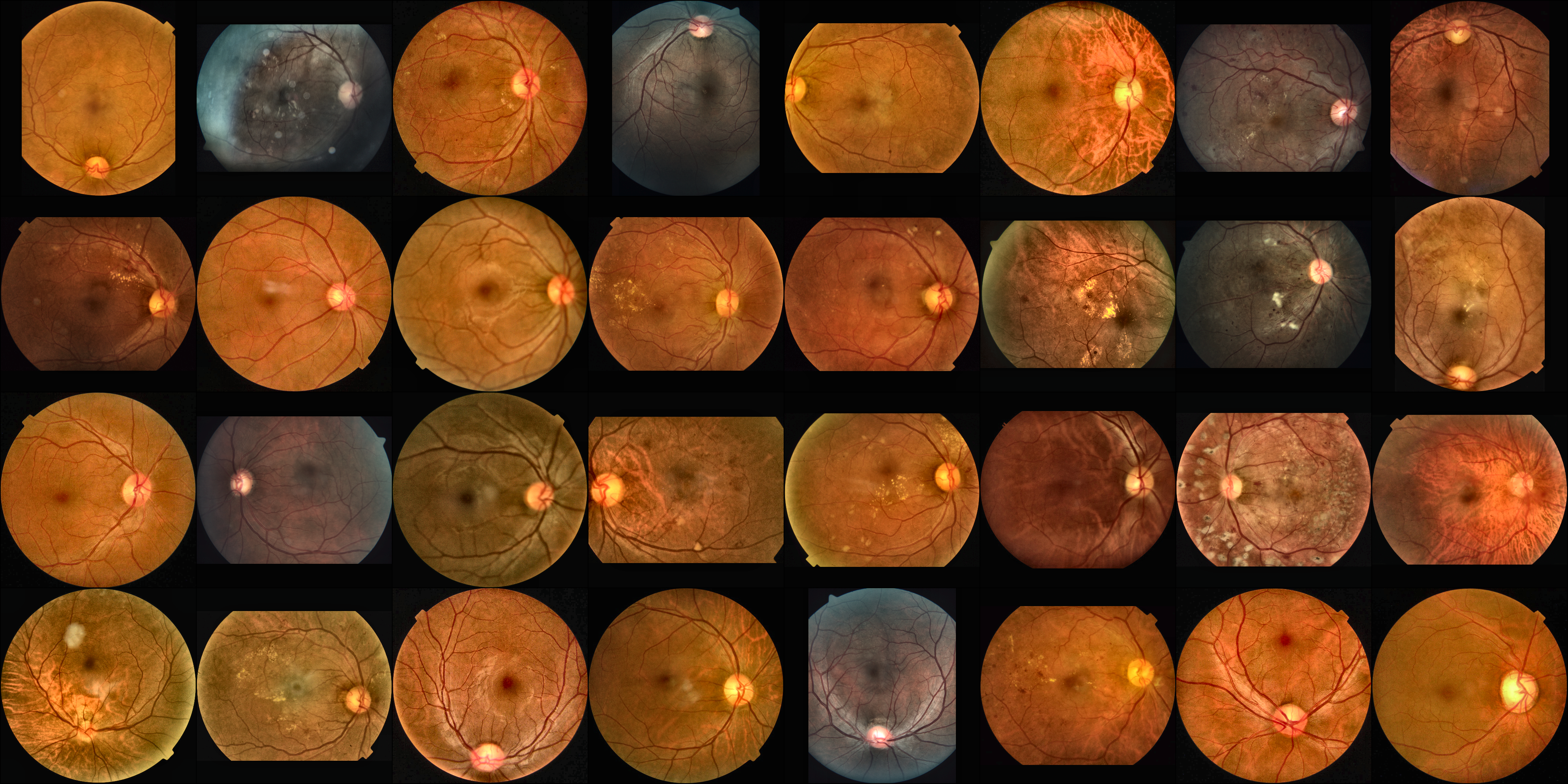
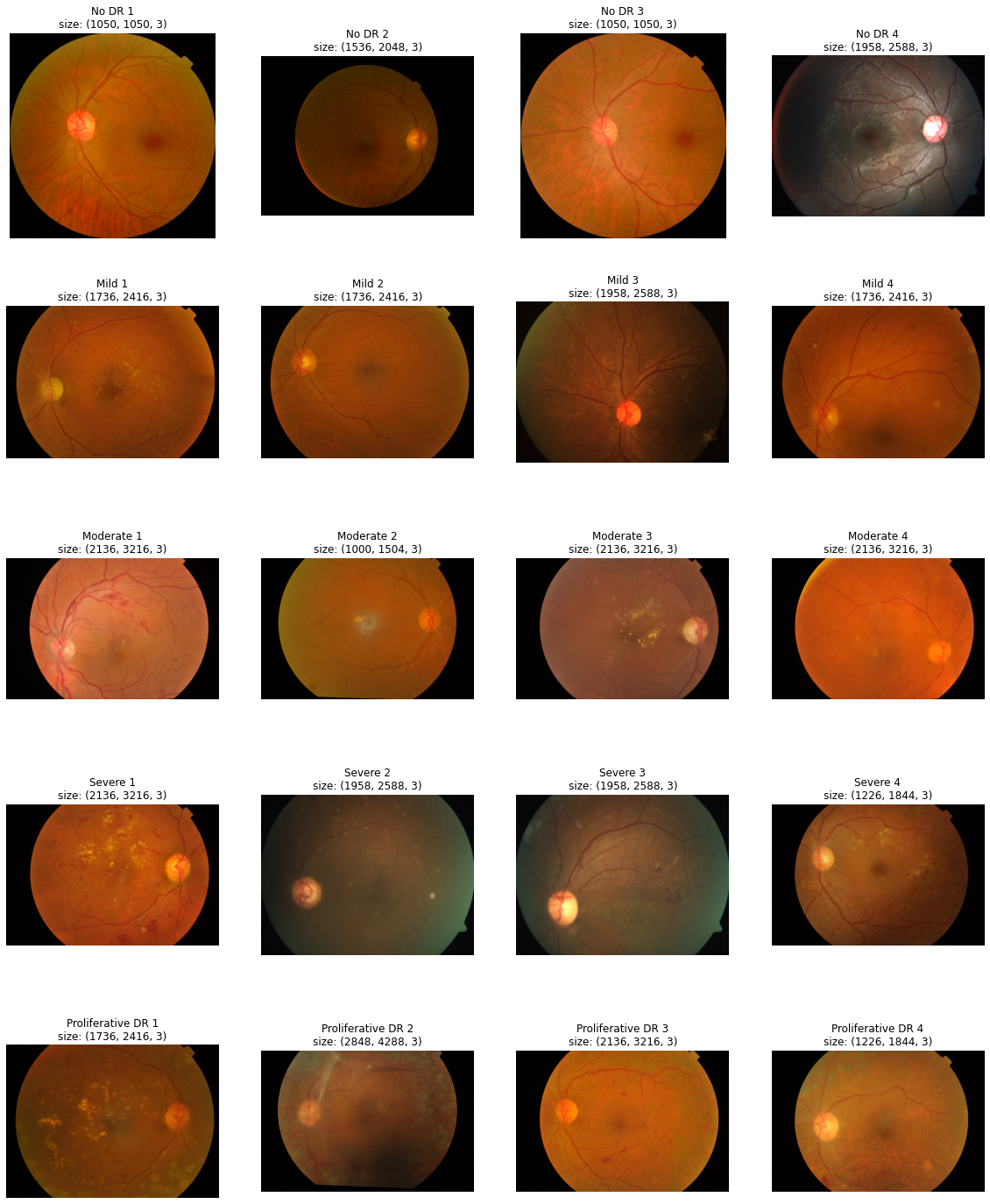
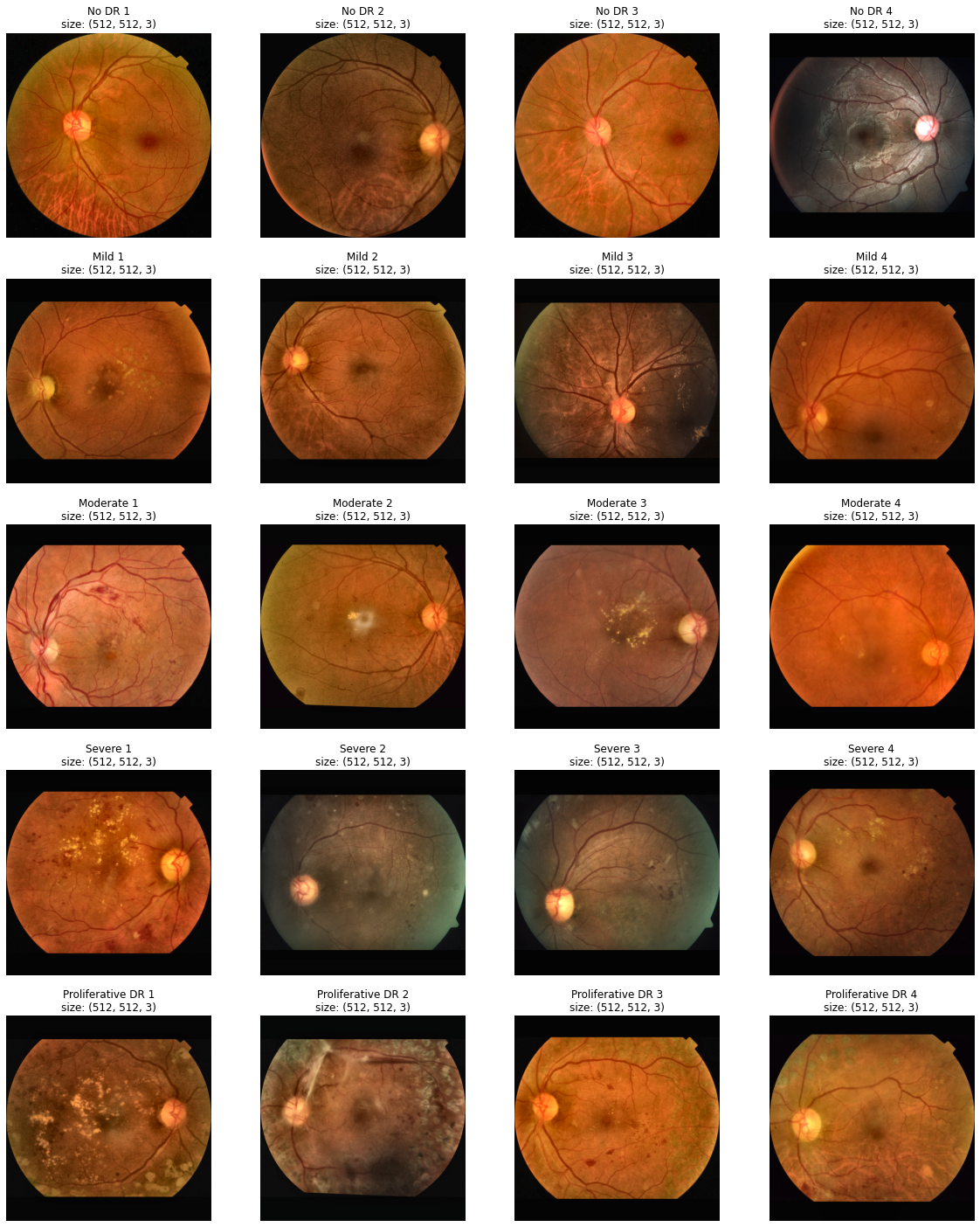
원본 데이터를 레이블 별로 확인해봅니다. Train data는 총 3662개, test data는 1928개가 있습니다. 아래는 각 레이블별 데이터의 개수입니다. 0에서 4로 갈수록 Diabetic retinopathy(DR, 당뇨성 망막증)의 병증이 악화됩니다. 전체 데이터 중 0(정상)의 비율이 50%로 다소 불균형한 데이터 분포를 보이고 있습니다. 또한, 아래 이미지를 보면 모든 데이터의 크기가 다른 것을 확인할 수 있습니다. 안저의 모양 역시 데이터별로 다릅니다.

0 - No DR / 1805개
1 - Mild / 370개
2 - Moderate / 999개
3 - Severe / 193개
4 - Proliferative DR / 295개
Total - 3662

1
2
3
4
5
6
7
8
9
10
11
12
13
14
fig , axes = plt.subplots(5,4)
fig.set_size_inches(20,25)
diagnosis = ["No DR", "Mild", "Moderate", "Severe", "Proliferative DR"]

for label in range(train_csv["diagnosis"].nunique()):
    random.seed(args["RANDOM_SEED"])
    filenames = random.sample(list(train_csv[train_csv["diagnosis"]==label]['id_code']), 4)
    for idx, file in enumerate(filenames):
        img = cv2.imread(args["TRAIN_IMGPATH"] + file + ".png", cv2.IMREAD_COLOR)
        img_size = img.shape
        img = cv2.cvtColor(img, cv2.COLOR_BGR2RGB)
        axes[label,idx%4].imshow(img)
        axes[label,idx%4].set_title(f"{diagnosis[label]} {idx+1}\nsize: {img_size}")
        axes[label,idx%4].axis('off')

png


Preprocess(Trim & Resize)

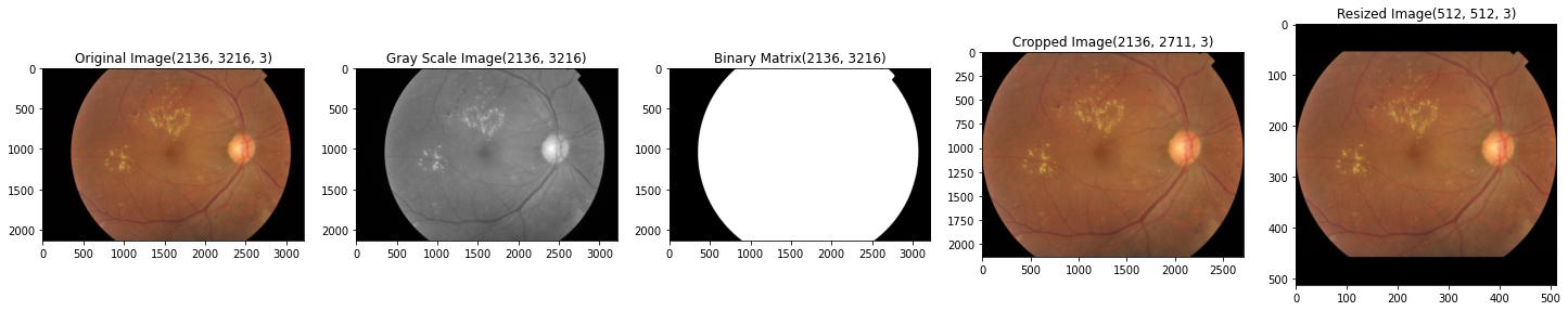
Original data를 봤을 때, 안저 좌우로 검은 배경이 존재하는 것을 확인할 수 있습니다. 모델이 최대한 동일한 형태의 안저 이미지를 학습할 수 있도록, 좌우 검정 배경을 제거하고 안저의 비율을 유지한 상태로 크기를 Resize 해주었습니다. 아래 두 함수를 통해 이러한 전처리를 적용하였습니다.

1
2
3
4
5
6
7
8
9
10
11
12
13
14
15
16
17
18
19
20
21
22
23
24
25
26
def trim(path):
    image = Image.open(path)
    image = np.array(image)
    percentage = 0.02
    img_gray = cv2.cvtColor(image, cv2.COLOR_RGB2GRAY)
    im = img_gray > 0.1* np.mean(img_gray[img_gray!=0]) # 0이 아닌 픽셀들의 평균의 10% 이상인 영역을 가져오기
    row_sums = np.sum(im, axis=1)
    col_sums = np.sum(im, axis=0)
    rows = np.where(row_sums > image.shape[1] * percentage)[0]
    cols = np.where(col_sums > image.shape[0] * percentage)[0]
    min_row, min_col = np.min(rows), np.min(cols)
    max_row, max_col = np.max(rows), np.max(cols)
    im_crop = image[min_row : max_row+1, min_col : max_col+1]
    return Image.fromarray(im_crop)

def resize_maintain_aspect(image, desired_size):
    """
    이미지 사이즈를 Resize할 때, Retina의 너비-높이 비율을 유지한다.
    """
    old_size = image.size
    ratio = float(desired_size) / max(old_size)
    new_size = tuple([int(x*ratio) for x in old_size])
    im2 = image.resize(new_size, Image.ANTIALIAS)
    new_im = Image.new("RGB", (desired_size, desired_size))
    new_im.paste(im2, ((desired_size - new_size[0]) // 2, (desired_size - new_size[1]) // 2))
    return new_im

1. View trimmed & resized data

전처리한 이미지를 확인합니다.

1
2
3
4
5
6
7
8
9
10
11
12
13
14
15
16
17
18
19
20
21
22
23
24
25
26
pth = glob.glob(args["TRAIN_IMGPATH"]+"*")
sample_path = pth[100]
image = Image.open(sample_path)
image = np.array(image)

percentage = 0.02
img_gray = cv2.cvtColor(image, cv2.COLOR_RGB2GRAY)
im = img_gray > 0.1* np.mean(img_gray[img_gray!=0]) # 0이 아닌 픽셀들의 평균의 10% 이상인 영역을 가져오기
row_sums = np.sum(im, axis=1)
col_sums = np.sum(im, axis=0)
rows = np.where(row_sums > image.shape[1] * percentage)[0]
cols = np.where(col_sums > image.shape[0] * percentage)[0]
min_row, min_col = np.min(rows), np.min(cols)
max_row, max_col = np.max(rows), np.max(cols)
im_crop = image[min_row : max_row+1, min_col : max_col+1]

image_crop = Image.fromarray(im_crop)
image_crop_not_maintain = cv2.resize(im_crop,(args["RESIZE"],args["RESIZE"]))

desired_size=args["RESIZE"]
old_size = image_crop.size
ratio = float(desired_size) / max(old_size)
new_size = tuple([int(x*ratio) for x in old_size])
im2 = image_crop.resize(new_size, Image.ANTIALIAS)
new_im = Image.new("RGB", (desired_size, desired_size))
new_im.paste(im2, ((desired_size - new_size[0]) // 2, (desired_size - new_size[1]) // 2))

(1) Trimming Process

1
2
3
4
5
6
7
8
9
10
11
12
13
fig , axes = plt.subplots(1,5)
fig.set_size_inches(25,5)

axes[0].imshow(image)
axes[0].set_title(f"Original Image{image.shape}")
axes[1].imshow(img_gray, cmap='gray')
axes[1].set_title(f"Gray Scale Image{img_gray.shape}")
axes[2].imshow(im, cmap='gray')
axes[2].set_title(f"Binary Matrix{im.shape}")
axes[3].imshow(im_crop)
axes[3].set_title(f"Cropped Image{im_crop.shape}")
axes[4].imshow(new_im)
axes[4].set_title(f"Resized Image{np.array(new_im).shape}")
1
Text(0.5, 1.0, 'Resized Image(512, 512, 3)')

png


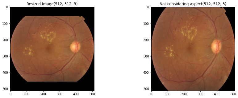
(2) Resize with its Aspect maintained

왼쪽 이미지는 안저 모양을 유지하면서 (512,512) 크기로 Resize해준 결과이고, 오른쪽 이미지는 검정 배경을 제거한 후, 바로 (512,512) 크기로 Resize한 결과입니다.

1
2
3
4
5
6
7
8
9
fig , axes = plt.subplots(1,2)
fig.set_size_inches(15,5)
"""
이미지 비율 유지
"""
axes[0].imshow(new_im)
axes[0].set_title(f"Resized Image{np.array(new_im).shape}")
axes[1].imshow(image_crop_not_maintain)
axes[1].set_title(f"Not considering aspect{image_crop_not_maintain.shape}")
1
Text(0.5, 1.0, 'Not considering aspect(512, 512, 3)')

png


(3) Trim + Resize + CLAHE

전처리 결과입니다. 모든 안저 이미지의 좌우 검정 배경이 제거되었고, 기존 안저의 모양은 유지하면서 크기가 (512,512)로 모두 맞춰진 것을 확인할 수 있습니다.

1
2
3
4
5
6
7
8
9
10
11
12
13
14
15
16
fig , axes = plt.subplots(5,4)
fig.set_size_inches(20,25)
diagnosis = ["No DR", "Mild", "Moderate", "Severe", "Proliferative DR"]

for label in range(train_csv["diagnosis"].nunique()):
    random.seed(args["RANDOM_SEED"])
    filenames = random.sample(list(train_csv[train_csv["diagnosis"]==label]['id_code']), 4)
    for idx, file in enumerate(filenames):
        
        img = trim(args["TRAIN_IMGPATH"] + file +'.png')
        img = np.array(resize_maintain_aspect(img, args['RESIZE']))
        img = A.CLAHE(p=1.0)(image = img)['image']
        img_size = img.shape
        axes[label,idx%4].imshow(img)
        axes[label,idx%4].set_title(f"{diagnosis[label]} {idx+1}\nsize: {img_size}")
        axes[label,idx%4].axis('off')

png


Transforms

Train 데이터셋에 적용되는 augmentation입니다. HorizontalFlip, VerticalFlip, RandomRotate90, CLAHE와 Normalize를 적용해주었습니다.

1
2
3
4
5
6
7
8
9
10
11
12
13
14
15
16
17
18
19
20
21
22
23
24
25
26
27
28
29
30
31
32
33
34
35
36
train_transforms = A.Compose([
#     A.Resize(width=args["RESIZE"], height=args["RESIZE"]),
    A.HorizontalFlip(p=0.5),
    A.VerticalFlip(p=0.5),
    A.RandomRotate90(p=0.5),
    A.CLAHE(p=1.0),
    A.Normalize(
        mean=[0.485, 0.456, 0.406],
        std=[0.229, 0.224, 0.225],
        max_pixel_value=255.0),
    ToTensorV2()
])

valid_transforms = A.Compose([
#     A.Resize(width=150, height=150),
    A.CLAHE(p=1.0),
    A.Normalize(
        mean=[0.485, 0.456, 0.406],
        std=[0.229, 0.224, 0.225],
        max_pixel_value=255.0),
    ToTensorV2()
])

# Augmentation결과 확인을 위한 transforms
check_train_transforms = A.Compose([
#     A.Resize(width=args["RESIZE"], height=args["RESIZE"]),
    A.HorizontalFlip(p=0.5),
    A.VerticalFlip(p=0.5),
    A.RandomRotate90(p=0.5),
    A.CLAHE(p=1.0),
    A.Normalize(
        mean=[0.0, 0.0, 0.0],
        std=[1.0, 1.0, 1.0],
        max_pixel_value=255.0),
    ToTensorV2()
])

Data Loader

데이터 로더 클래스를 정의합니다. 사전에 이미지를 np 형태로 저장해놓았고, 이를 불러오게끔 코드로 처리하였습니다.

1
2
3
4
5
6
7
8
9
10
11
12
13
14
15
16
17
class RETINANPDataset(Dataset):
    def __init__(self, np_array, label_np, transform=None):
        super().__init__()
        self.np_array = np_array
        self.label_np = label_np
        self.transform = transform
    
    def __getitem__(self, index):
        image = self.np_array[index]
        label = self.label_np[index]
        if self.transform:
            image = self.transform(image=image)["image"]
            
        return image, label, label
            
    def __len__(self):
        return self.np_array.shape[0]

데이터셋 나누기

train과 valid 데이터는 8:2의 비율로 각 레이블별 비율을 유지하면서 나누어 주었습니다.

1
2
3
4
5
# (512,512)
train_np = np.load("../input/blindness-experiment-trim/train_trim_np.npy")
label_np = np.load("../input/blindness-experiment-trim/train_trim_label.npy")

X_train, X_valid, y_train, y_valid = train_test_split(train_np,label_np, test_size=0.2,random_state=42, stratify=label_np)

데이터셋 나누기

데이터 로더를 적용하여 Train, Valid, Test셋을 배치 형태로 만들어 줍니다.

1
2
3
4
5
6
7
8
9
10
11
12
13
14
15
16
17
18
19
20
21
22
23
# Using saved Numpy data
train_dataset = RETINANPDataset(np_array = X_train,
                              label_np = y_train, 
                              transform=train_transforms)

valid_dataset = RETINANPDataset(np_array=X_valid,
                            label_np= y_valid,
                            transform=valid_transforms)

test_dataset = RETINADataset(dataframe=test_csv,
                            image_path= args["TEST_IMGPATH"],
                            transform=valid_transforms)

train_loader = DataLoader(train_dataset, batch_size=args["BATCH_SIZE"], num_workers=2, shuffle=True)
valid_loader = DataLoader(valid_dataset, batch_size=args["BATCH_SIZE"], num_workers=2, shuffle=False)
test_loader = DataLoader(test_dataset, batch_size=args["BATCH_SIZE"], num_workers=2, shuffle=False)


train_dataset_check = RETINANPDataset(np_array = X_train,
                              label_np = y_train, 
                              transform=check_train_transforms)

train_loader_check = DataLoader(train_dataset_check, batch_size=args["BATCH_SIZE"], num_workers=2, shuffle=True)

Check Augmentations in Data Loader

최종적으로 데이터로더를 통해 학습되는 데이터를 확인합니다.

1
2
3
4
5
6
for X,y,y in train_loader_check:
    save_image(X,"./aug_check.png")
    print(f"Shape of Batch Data: {X.shape}")
    break

Image.open("./aug_check.png")
1
Shape of Batch Data: torch.Size([32, 3, 512, 512])

png


Utils

대회의 평가 지표는 Quadratic weighted kappa(QWK)입니다. 간단히 설명하자면 이 평가지표에서는 실제 레이블에서 모델의 예측값이 멀어질수록 더 큰 loss를 줍니다. 모델이 레이블에 최대한 가까운 예측값을 추출할 수 있도록 학습시켜야하기 때문에, MSE Loss를 사용했습니다. 아래 표는 Trim 전처리와 (150,150) Resize만 하여 모델을 학습시켜본 결과입니다. Crossentropy loss를 사용했을때보다 MSE Loss를 사용했을 때 valid 데이터와 test 데이터에서 더 좋은 결과를 보여주었습니다.

Model Loss Private Score Public Score Valid QWK Valid Loss
ResNet18 MSE 0.7610 0.5091 0.8599 0.4247
ResNet18 CrossEntropy 0.7183 0.4173 0.8142 0.6464

1
2
3
4
5
6
7
8
9
10
11
12
13
14
15
16
17
18
19
20
21
22
23
24
25
def make_predictions(model, loader, output_csv='submission.csv'):
    preds = []
    filenames = []
    model.eval()
    
    for X,y, files in tqdm(loader):
        X = X.to(args["DEVICE"])
        with torch.no_grad():
            pred = model(X)
            pred[pred < 0.5] = 0
            pred[(pred >= 0.5) & (pred < 1.5)] = 1
            pred[(pred >= 1.5) & (pred < 2.5)] = 2
            pred[(pred >= 2.5) & (pred < 3.5)] = 3
            pred[(pred >= 3.5)] = 4
            pred = pred.squeeze(1)
            preds.append(pred.cpu().numpy().astype(np.int64))
            filenames.append(files)
            
    preds = [i for j in preds for i in j]
    filenames = [val for sublist in filenames for val in sublist]
    
    df = pd.DataFrame({"id_code" : filenames, "diagnosis" : preds})
    df.to_csv(output_csv, index=False)
    model.train()
    print("Prediction Finished.. ")
1
2
3
4
5
6
7
8
9
10
11
12
13
14
15
16
17
18
19
20
21
22
23
24
25
26
27
28
29
30
31
32
33
34
35
36
37
def validation(loader, model, criterion, device=args["DEVICE"]):
    model.eval()
    val_losses = []
    all_preds, all_labels =[], []
    num_correct = 0
    num_samples = 0
    
    for X, y, files in tqdm(loader):
        X = X.to(device)
        y = y.to(device)
        
        with torch.no_grad():
            pred = model(X)
            loss = criterion(pred, y.unsqueeze(1).float())
            
        pred[pred < 0.5] = 0
        pred[(pred >= 0.5) & (pred < 1.5)] = 1
        pred[(pred >= 1.5) & (pred < 2.5)] = 2
        pred[(pred >= 2.5) & (pred < 3.5)] = 3
        pred[(pred >= 3.5)] = 4
        pred = pred.long().view(-1)
        y = y.view(-1)

            
#         _, predictions = scores.max(1)
        num_correct += (pred==y).sum()
        num_samples += pred.shape[0]
        
        all_preds.append(pred.detach().cpu().numpy())
        all_labels.append(y.detach().cpu().numpy())
        val_losses.append(loss.item())

    val_accuracy = "{:.6f}".format(num_correct/num_samples)
    val_loss_total = "{:.6f}".format(sum(val_losses)/len(val_losses))
    model.train()
    
    return np.concatenate(all_preds, axis=0), np.concatenate(all_labels, axis=0), np.float(val_accuracy), np.float(val_loss_total)
1
2
3
4
5
6
7
def load_checkpoint(checkpoint, model, optimizer, lr):
    model.load_state_dict(checkpoint["state_dict"])
    optimizer.load_state_dict(checkpoint["optimizer"])
    
    for param_groups in optimizer.param_groups:
        param_groups["lr"] = lr
    print("Loaded Checkpoint.. ")

Train

학습 함수입니다.

1
2
3
4
5
6
7
8
9
10
11
12
13
14
15
16
17
18
19
20
21
22
23
def train_one_epoch(model, loader, optimizer, criterion, scaler, device):
    
    losses = []
    loop = tqdm(loader)
    
    for idx, (X, y, _) in enumerate(loop):
        
        X = X.to(device=device)
        y = y.to(device=device)
        
        with torch.cuda.amp.autocast():
            scores = model(X)
            loss = criterion(scores, y.unsqueeze(1).float())
        
        losses.append(loss.item())
        optimizer.zero_grad()
        scaler.scale(loss).backward()
        scaler.step(optimizer)
        scaler.update()
        loop.set_postfix(loss=loss.item())
    print(f"Loss average over Epoch : {sum(losses)/len(losses)}")
    
    return "{:.6f}".format(sum(losses)/len(losses))

SE Block

ResNet18에 Squeeze and Excitation Block(SE Block)을 추가했습니다. SE Block을 통해 Convolution 연산을 거친 피쳐맵에서 중요한 정보들을 압축(Squeeze)하고 재조정(Recalibration)할 수 있습니다. 중요 정보를 추출하는 과정에서는 GAP(Global Average Pooling)을 사용하고, 재조정 과정에서는 Fully Connected Layer과 비선형 함수인 ReLU, Sigmoid이 사용됩니다. 결국 SE Block을 거치게 되면 피쳐맵이 채널들의 중요도에 따라 스케일 됩니다.

실제 아래 실험 결과표에서 확인할 수 있듯이, ResNet18 모델 구조에 SEBlock을 추가했을 경우 test셋에 대한 Quadratic Weighted Kappa 점수가 더 높은 것을 확인할 수 있습니다.

Model Loss Private Score Public Score Valid QWK Valid Loss
ResNet18 MSE 0.7610 0.5091 0.8599 0.4247
ResNet18 + SEBlock MSE 0.8310 0.6766 0.8491 0.4059

Squeeze and Excitation에 대한 더 자세한 설명은 아래 블로그를 참고하시면 됩니다.


1
2
3
4
5
6
7
8
9
10
11
12
13
14
15
16
17
18
19
20
21
22
23
class SE(nn.Module):

    def __init__(self, num_channels, reduction_ratio=2):
        super().__init__()
        num_channels_reduced = num_channels // reduction_ratio
        self.reduction_ratio = reduction_ratio
        self.fc1 = nn.Linear(num_channels, num_channels_reduced, bias=True)
        self.fc2 = nn.Linear(num_channels_reduced, num_channels, bias=True)
        self.relu = nn.ReLU()
        self.sigmoid = nn.Sigmoid()

    def forward(self, input_tensor):
        batch_size, num_channels, H, W = input_tensor.size()
        # Average along each channel
        squeeze_tensor = input_tensor.view(batch_size, num_channels, -1).mean(dim=2)

        # channel excitation
        fc_out_1 = self.relu(self.fc1(squeeze_tensor))
        fc_out_2 = self.sigmoid(self.fc2(fc_out_1))

        a, b = squeeze_tensor.size()
        output_tensor = torch.mul(input_tensor, fc_out_2.view(a, b, 1, 1))
        return output_tensor

SE Block을 ResNet18 모델 구조에 추가하기

1
2
3
4
5
6
7
8
9
10
11
12
13
14
15
16
17
18
19
20
21
22
23
24
25
26
27
28
29
30
31
32
33
34
35
36
37
38
39
40
41
42
43
44
45
46
47
48
49
50
51
52
53
54
55
56
57
58
59
60
61
62
63
64
65
66
67
68
69
70
71
72
73
74
75
76
77
def get_model():
    
    if args["MODEL_VER"]==18:
        try:
            model = models.resnet18(pretrained=True)
        except:
            model = models.resnet18(pretrained=False)
            model.load_state_dict(torch.load("../input/pretrained-pytorch-models/resnet18-5c106cde.pth"))

        if args["SEBLOCK"]:
            for i in range(len(model.layer1)):
                model.layer1[i].se = SE(64)

            for i in range(len(model.layer2)):
                model.layer2[i].se = SE(128)

            for i in range(len(model.layer3)):
                model.layer3[i].se = SE(256)

            for i in range(len(model.layer4)):
                model.layer4[i].se = SE(512)
            print("Squeeze & Excitation Networks applied.. ")
            
        model.fc = nn.Linear(512, 1)
        model = model.to(args["DEVICE"])
        
    elif args["MODEL_VER"]==50:
        try:
            model = models.resnet50(pretrained=True)
        except:
            model = models.resnet50(pretrained=False)
            model.load_state_dict(torch.load("../input/pretrained-pytorch-models/resnet50-19c8e357.pth"))

        if args["SEBLOCK"]:
            for i in range(len(model.layer3)):
                model.layer3[i].se = SE(1024)

            for i in range(len(model.layer2)):
                model.layer2[i].se = SE(512)

            for i in range(len(model.layer1)):
                model.layer1[i].se = SE(256)

            for i in range(len(model.layer4)):
                model.layer4[i].se = SE(2048)
            print("Squeeze & Excitation Networks applied.. ")

        for param in model.parameters():
            param.requires_grad = True  

        model.fc = nn.Linear(2048, 1)
        model = model.to(args["DEVICE"])
    else:
        try:
            model = models.resnext50_32x4d(pretrained=True)
        except:
            model = models.resnext50_32x4d(pretrained=False)
            model.load_state_dict(torch.load("../input/pytorch-resnext50-pretrained-model/resnext50_32x4d-7cdf4587.pth"))

        if args["SEBLOCK"]:
            for i in range(len(model.layer1)):
                model.layer1[i].se = SE(256)
            for i in range(len(model.layer2)):
                model.layer2[i].se = SE(512)
            for i in range(len(model.layer3)):
                model.layer3[i].se = SE(1024)
            for i in range(len(model.layer4)):
                model.layer4[i].se = SE(2048)
            print("Squeeze & Excitation Networks applied.. ")

        for param in model.parameters():
            param.requires_grad = True 
            
        model.fc = nn.Linear(2048, 1)
        model = model.to(args["DEVICE"])

    return model

전체 학습 함수

학습 함수 코드입니다. Automatic Mixed Precision을 적용했습니다. AMP를 사용하였을 때의 장점은 아래와 같습니다.

  • 처리 속도를 높이기 위한 FP16(16bit floating point)연산과 정확도 유지를 위한 FP32 연산을 섞어 학습하는 방법.
  • Tensor Core를 활용한 FP16연산을 이용하면 FP32연산 대비 절반의 메모리 사용량과 8배의 연산 처리량 & 2배의 메모리 처리량 효과가 있음.
1
2
3
4
5
6
7
8
9
10
11
12
13
14
15
16
17
18
19
20
21
22
23
24
25
26
27
28
29
30
31
32
33
34
35
36
37
38
39
40
41
42
43
44
45
46
47
48
49
50
51
52
53
54
def train():
    model = get_model()
    criterion = nn.MSELoss()
    optimizer = torch.optim.Adam(model.parameters(), lr=args["LEARNING_RATE"], weight_decay=args["WEIGHT_DECAY"]) 
    '''
    Automatic Mixed Precision(amp)
    '''
    scaler = torch.cuda.amp.GradScaler()
    best_val = np.inf
    early_stopping_count = 0
    
    if args["LOAD_MODEL"] and args["CHECKPOINT_FILE"] in os.listdir():
        load_checkpoint(torch.load(args["CHECKPOINT_FILE"]), model, optimizer, args["LEARNING_RATE"])
    
    for epoch in range(args["NUM_EPOCHS"]):
        train_loss = train_one_epoch(model, train_loader, optimizer, criterion, scaler, args["DEVICE"])
        
        preds, labels, val_accuarcy, val_loss = validation(valid_loader, model, criterion, device=args["DEVICE"])
        
        print("Epoch: {}/{}.. ".format(epoch + 1, args['NUM_EPOCHS']) +
              "Training Loss: {}.. ".format(train_loss) +
              "Valid Accuracy: {}.. ".format(val_accuarcy) + 
              "Valid Loss: {}.. ".format(val_loss) +
              "Valid QWK: {:.6f}.. ".format(cohen_kappa_score(labels, preds, weights='quadratic')))
        
        # Save Model
        if val_loss < best_val:
            print(f"Valid Loss improved from {best_val} -> {val_loss}")
            best_val = val_loss
            
            checkpoint = {
                "state_dict": model.state_dict(),
                "optimizer": optimizer.state_dict()
            }      
            try:
                os.remove(f_pth)
            except:
                pass
            
            torch.save(checkpoint, f"{args['CHECKPOINT_FILE']}")

            f_pth =  f"{args['CHECKPOINT_FILE']}"
            
            early_stopping_count=0
            
        else:
            early_stopping_count+=1
            print(f"Valid Loss did not improved from {best_val}.. Counter {early_stopping_count}/{args['EARLY_STOPPING']} ")
            
            if early_stopping_count>args["EARLY_STOPPING"]:
                print("Early Stopped ..")
                break


학습시키기

랜덤 시드를 고정시키고 학습 시킵니다.

1
2
3
4
5
6
seed=42
torch.manual_seed(seed)
torch.cuda.manual_seed_all(seed)
torch.backends.cudnn.deterministic = True
torch.backends.cudnn.benchmark = False
train()
1
2
3
4
5
6
7
8
9
10
11
12
13
14
15
16
17
18
19
20
21
22
23
24
25
26
27
28
29
30
31
32
33
34
35
36
37
38
39
40
41
42
43
44
45
46
47
48
49
50
51
52
53
54
55
56
57
58
59
60
61
62
63
64
65
66
67
68
69
70
71
72
73
74
75
76
77
78
79
80
81
82
83
84
85
86
87
88
89
90
91
92
93
94
95
96
97
98
99
100
101
102
103
104
105
106
107
108
109
110
111
112
113
114
115
116
117
118
119
120
121
122
123
124
125
126
127
128
129
130
131
132
133
134
135
136
137
138
139
140
141
142
143
144
145
146
147
148
149
150
151
152
153
154
155
156
157
158
159
160
161
162
163
164
165
166
167
168
169
170
171
172
173
174
175
176
177
178
179
180
181
182
183
184
185
186
187
188
189
190
191
192
193
194
195
196
197
198
199
200
201
202
203
204
205
206
207
208
209
210
211
212
213
214
215
216
217
218
219
220
221
222
223
224
225
226
227
228
229
230
231
232
233
234
235
236
237
238
239
240
241
242
243
244
245
246
247
248
249
250
251
Downloading: "https://download.pytorch.org/models/resnext50_32x4d-7cdf4587.pth" to /root/.cache/torch/hub/checkpoints/resnext50_32x4d-7cdf4587.pth


Squeeze & Excitation Networks applied.. 


100%|██████████| 92/92 [01:57<00:00,  1.28s/it, loss=0.819]
  0%|          | 0/23 [00:00<?, ?it/s]

Loss average over Epoch : 1.3487307510298232


100%|██████████| 23/23 [00:01<00:00, 12.19it/s]


Epoch: 1/100.. Training Loss: 1.348731.. Valid Accuracy: 0.560709.. Valid Loss: 0.575182.. Valid QWK: 0.798112.. 
Valid Loss improved from inf -> 0.575182


100%|██████████| 92/92 [01:56<00:00,  1.27s/it, loss=0.566]
  0%|          | 0/23 [00:00<?, ?it/s]

Loss average over Epoch : 0.5655950175841218


100%|██████████| 23/23 [00:02<00:00,  9.81it/s]


Epoch: 2/100.. Training Loss: 0.565595.. Valid Accuracy: 0.68895.. Valid Loss: 0.448546.. Valid QWK: 0.855907.. 
Valid Loss improved from 0.575182 -> 0.448546


100%|██████████| 92/92 [01:56<00:00,  1.27s/it, loss=0.257]
  0%|          | 0/23 [00:00<?, ?it/s]

Loss average over Epoch : 0.5029683655694775


100%|██████████| 23/23 [00:02<00:00, 11.33it/s]


Epoch: 3/100.. Training Loss: 0.502968.. Valid Accuracy: 0.712142.. Valid Loss: 0.424432.. Valid QWK: 0.864212.. 
Valid Loss improved from 0.448546 -> 0.424432


100%|██████████| 92/92 [01:56<00:00,  1.27s/it, loss=0.607]
  0%|          | 0/23 [00:00<?, ?it/s]

Loss average over Epoch : 0.42268620949724445


100%|██████████| 23/23 [00:02<00:00,  9.28it/s]
  0%|          | 0/92 [00:00<?, ?it/s]

Epoch: 4/100.. Training Loss: 0.422686.. Valid Accuracy: 0.693042.. Valid Loss: 0.587159.. Valid QWK: 0.758567.. 
Valid Loss did not improved from 0.424432.. Counter 1/10 


100%|██████████| 92/92 [01:56<00:00,  1.27s/it, loss=0.376]
  0%|          | 0/23 [00:00<?, ?it/s]

Loss average over Epoch : 0.41506120708325633


100%|██████████| 23/23 [00:02<00:00,  8.39it/s]
  0%|          | 0/92 [00:00<?, ?it/s]

Epoch: 5/100.. Training Loss: 0.415061.. Valid Accuracy: 0.731241.. Valid Loss: 0.425504.. Valid QWK: 0.843659.. 
Valid Loss did not improved from 0.424432.. Counter 2/10 


100%|██████████| 92/92 [01:57<00:00,  1.27s/it, loss=1.27]
  0%|          | 0/23 [00:00<?, ?it/s]

Loss average over Epoch : 0.4283194863439902


100%|██████████| 23/23 [00:01<00:00, 12.55it/s]
  0%|          | 0/92 [00:00<?, ?it/s]

Epoch: 6/100.. Training Loss: 0.428319.. Valid Accuracy: 0.656207.. Valid Loss: 0.59253.. Valid QWK: 0.828938.. 
Valid Loss did not improved from 0.424432.. Counter 3/10 


100%|██████████| 92/92 [01:56<00:00,  1.27s/it, loss=0.355]
  0%|          | 0/23 [00:00<?, ?it/s]

Loss average over Epoch : 0.402648795881997


100%|██████████| 23/23 [00:02<00:00, 10.60it/s]
  0%|          | 0/92 [00:00<?, ?it/s]

Epoch: 7/100.. Training Loss: 0.402649.. Valid Accuracy: 0.744884.. Valid Loss: 0.528034.. Valid QWK: 0.786981.. 
Valid Loss did not improved from 0.424432.. Counter 4/10 


100%|██████████| 92/92 [01:57<00:00,  1.27s/it, loss=0.666]
  0%|          | 0/23 [00:00<?, ?it/s]

Loss average over Epoch : 0.45209699950140453


100%|██████████| 23/23 [00:01<00:00, 12.23it/s]


Epoch: 8/100.. Training Loss: 0.452097.. Valid Accuracy: 0.698499.. Valid Loss: 0.409218.. Valid QWK: 0.850001.. 
Valid Loss improved from 0.424432 -> 0.409218


100%|██████████| 92/92 [01:57<00:00,  1.28s/it, loss=0.676]
  0%|          | 0/23 [00:00<?, ?it/s]

Loss average over Epoch : 0.4371181230020264


100%|██████████| 23/23 [00:01<00:00, 12.17it/s]
  0%|          | 0/92 [00:00<?, ?it/s]

Epoch: 9/100.. Training Loss: 0.437118.. Valid Accuracy: 0.462483.. Valid Loss: 0.622757.. Valid QWK: 0.756151.. 
Valid Loss did not improved from 0.409218.. Counter 1/10 


100%|██████████| 92/92 [01:57<00:00,  1.27s/it, loss=0.665]
  0%|          | 0/23 [00:00<?, ?it/s]

Loss average over Epoch : 0.42180322904301726


100%|██████████| 23/23 [00:01<00:00, 12.54it/s]
  0%|          | 0/92 [00:00<?, ?it/s]

Epoch: 10/100.. Training Loss: 0.421803.. Valid Accuracy: 0.529332.. Valid Loss: 0.528666.. Valid QWK: 0.803896.. 
Valid Loss did not improved from 0.409218.. Counter 2/10 


100%|██████████| 92/92 [01:56<00:00,  1.27s/it, loss=0.306]
  0%|          | 0/23 [00:00<?, ?it/s]

Loss average over Epoch : 0.4050265988739936


100%|██████████| 23/23 [00:01<00:00, 12.90it/s]
  0%|          | 0/92 [00:00<?, ?it/s]

Epoch: 11/100.. Training Loss: 0.405027.. Valid Accuracy: 0.74352.. Valid Loss: 0.63127.. Valid QWK: 0.746908.. 
Valid Loss did not improved from 0.409218.. Counter 3/10 


100%|██████████| 92/92 [01:57<00:00,  1.28s/it, loss=0.846]
  0%|          | 0/23 [00:00<?, ?it/s]

Loss average over Epoch : 0.42884239845949673


100%|██████████| 23/23 [00:01<00:00, 11.76it/s]
  0%|          | 0/92 [00:00<?, ?it/s]

Epoch: 12/100.. Training Loss: 0.428842.. Valid Accuracy: 0.675307.. Valid Loss: 0.74766.. Valid QWK: 0.692850.. 
Valid Loss did not improved from 0.409218.. Counter 4/10 


100%|██████████| 92/92 [01:58<00:00,  1.28s/it, loss=0.657]
  0%|          | 0/23 [00:00<?, ?it/s]

Loss average over Epoch : 0.39752021772058116


100%|██████████| 23/23 [00:02<00:00,  7.80it/s]
  0%|          | 0/92 [00:00<?, ?it/s]

Epoch: 13/100.. Training Loss: 0.397520.. Valid Accuracy: 0.466576.. Valid Loss: 0.602466.. Valid QWK: 0.723202.. 
Valid Loss did not improved from 0.409218.. Counter 5/10 


100%|██████████| 92/92 [01:57<00:00,  1.27s/it, loss=1.03]
  0%|          | 0/23 [00:00<?, ?it/s]

Loss average over Epoch : 0.39626112070096575


100%|██████████| 23/23 [00:02<00:00,  8.71it/s]
  0%|          | 0/92 [00:00<?, ?it/s]

Epoch: 14/100.. Training Loss: 0.396261.. Valid Accuracy: 0.740791.. Valid Loss: 0.504398.. Valid QWK: 0.813603.. 
Valid Loss did not improved from 0.409218.. Counter 6/10 


100%|██████████| 92/92 [01:57<00:00,  1.28s/it, loss=0.812]
  0%|          | 0/23 [00:00<?, ?it/s]

Loss average over Epoch : 0.43474946964694106


100%|██████████| 23/23 [00:02<00:00, 10.29it/s]
  0%|          | 0/92 [00:00<?, ?it/s]

Epoch: 15/100.. Training Loss: 0.434749.. Valid Accuracy: 0.676671.. Valid Loss: 0.434476.. Valid QWK: 0.827332.. 
Valid Loss did not improved from 0.409218.. Counter 7/10 


100%|██████████| 92/92 [01:56<00:00,  1.27s/it, loss=0.467]
  0%|          | 0/23 [00:00<?, ?it/s]

Loss average over Epoch : 0.44178698454862053


100%|██████████| 23/23 [00:01<00:00, 12.01it/s]
  0%|          | 0/92 [00:00<?, ?it/s]

Epoch: 16/100.. Training Loss: 0.441787.. Valid Accuracy: 0.652115.. Valid Loss: 0.457748.. Valid QWK: 0.829874.. 
Valid Loss did not improved from 0.409218.. Counter 8/10 


100%|██████████| 92/92 [01:56<00:00,  1.27s/it, loss=0.477]
  0%|          | 0/23 [00:00<?, ?it/s]

Loss average over Epoch : 0.3990700281346622


100%|██████████| 23/23 [00:02<00:00, 11.46it/s]
  0%|          | 0/92 [00:00<?, ?it/s]

Epoch: 17/100.. Training Loss: 0.399070.. Valid Accuracy: 0.706685.. Valid Loss: 0.460656.. Valid QWK: 0.821181.. 
Valid Loss did not improved from 0.409218.. Counter 9/10 


100%|██████████| 92/92 [01:57<00:00,  1.28s/it, loss=0.272]
  0%|          | 0/23 [00:00<?, ?it/s]

Loss average over Epoch : 0.40094906269856123


100%|██████████| 23/23 [00:01<00:00, 12.13it/s]
  0%|          | 0/92 [00:00<?, ?it/s]

Epoch: 18/100.. Training Loss: 0.400949.. Valid Accuracy: 0.622101.. Valid Loss: 0.544332.. Valid QWK: 0.795611.. 
Valid Loss did not improved from 0.409218.. Counter 10/10 


100%|██████████| 92/92 [01:56<00:00,  1.27s/it, loss=0.247]
  0%|          | 0/23 [00:00<?, ?it/s]

Loss average over Epoch : 0.4187986902568651


100%|██████████| 23/23 [00:02<00:00, 11.36it/s]

Epoch: 19/100.. Training Loss: 0.418799.. Valid Accuracy: 0.618008.. Valid Loss: 0.46466.. Valid QWK: 0.837597.. 
Valid Loss did not improved from 0.409218.. Counter 11/10 
Early Stopped ..

Test

Test셋에 대한 예측과 예측 결과값을 submission.csv에 저장합니다.

1
2
3
4
5
6
7
8
def test():
    model = get_model()
    optimizer = torch.optim.Adam(model.parameters(), lr=args["LEARNING_RATE"], weight_decay=args["WEIGHT_DECAY"]) 

    load_checkpoint(torch.load("./" + args['CHECKPOINT_FILE']), model, optimizer, args["LEARNING_RATE"])

    make_predictions(model, test_loader, output_csv='submission.csv')
    
1
2
3
test()
sub_test = pd.read_csv("./submission.csv")
sub_test
1
2
3
4
5
6
7
8
9
10
11
12
13
14
15
Downloading: "https://download.pytorch.org/models/resnext50_32x4d-7cdf4587.pth" to /root/.cache/torch/hub/checkpoints/resnext50_32x4d-7cdf4587.pth


Squeeze & Excitation Networks applied.. 


  0%|          | 0/61 [00:00<?, ?it/s]

Loaded Checkpoint.. 


100%|██████████| 61/61 [02:44<00:00,  2.69s/it]


Prediction Finished.. 
id_code diagnosis
0 0005cfc8afb6 2
1 003f0afdcd15 2
2 006efc72b638 2
3 00836aaacf06 2
4 009245722fa4 3
... ... ...
1923 ff2fd94448de 3
1924 ff4c945d9b17 2
1925 ff64897ac0d8 2
1926 ffa73465b705 2
1927 ffdc2152d455 1

1928 rows × 2 columns


결론

이번 프로젝트에서는 pre-trained ResNet18에 SEBlock을 적용한 베이스라인 모델을 만들었습니다. 이후 하이퍼파라미터 튜닝 및 다른 모델 구조들을 적용하여 점수를 높일 수 있습니다. 현재 학습에는 동일한 random seed로 train과 valid를 8:2로 나눈 데이터셋을 사용했는데, 5-fold cross validation과 soft-voting과 같은 방식으로 여러 모델을 앙상블하여 더욱 강건한 예측값을 뽑아낼 수도 있을 것으로 기대합니다. 또한 https://www.kaggle.com/c/diabetic-retinopathy-detection/data 대회에서 제공하고 있는 약 35,000개의 Fundus 이미지를 학습한 모델에 transfer learning을 시켜주어 정확도를 더 높일 수도 있을 것입니다.


참고 자료

[1] Squeeze and Excitation Block (1): https://github.com/edshkim98/ChannelwiseAttention/blob/main/resnet_se.py
[2] Squeeze and Excitation Block (2): https://jayhey.github.io/deep%20learning/2018/07/18/SENet/
[3] Quadratic Weighted Kappa: https://www.kaggle.com/aroraaman/quadratic-kappa-metric-explained-in-5-simple-steps
[4] https://arxiv.org/abs/1709.01507

0%