Cut Mix 방법 소개
Invasive Species Monitoring
Identify images of invasive hydrangea
https://www.kaggle.com/c/invasive-species-monitoring
평가 지표 : Area under ROC Curve
패키지 불러오기
필요한 라이브러라들을 불러옵니다.
1 | |
하이퍼 파라미터
하이퍼파라미터 값들이 있는 딕셔너리를 정해줍니다.
1 | |
데이터 불러오기
데이터를 간단히 살펴보면, invasive(1) 데이터는 1,448개, non-invasive(0) 데이터는 847개 입니다. 또한 예측에 사용될 Test 데이터는 전체 1,531개 입니다. 학습 데이터 전체를 사용하기 위해, 5-Fold Stratify로 모델을 훈련합니다.
1 | |
1 | |
| name | invasive | path | |
|---|---|---|---|
| 0 | 1 | 0 | ../input/invasivespecies/train/1.jpg |
| 1 | 2 | 0 | ../input/invasivespecies/train/2.jpg |
| 2 | 3 | 1 | ../input/invasivespecies/train/3.jpg |
| 3 | 4 | 0 | ../input/invasivespecies/train/4.jpg |
| 4 | 5 | 1 | ../input/invasivespecies/train/5.jpg |
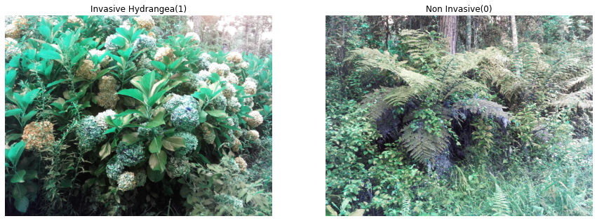
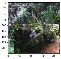
Invasive(1)/Non-invasive(0) 이미지 확인
침입종 수국(1)과 침입종이 아닌 식물(0)의 이미지입니다.
데이터 로더
데이터 로더 클래스를 정의합니다.
1 | |
Transforms 함수 정의
Train 데이터에 적용된 augmentation : RandomResizedCrop & RandomHorizontalFlip
Valid 데이터에 적용된 augmentation : Resize & CenterCrop
위 augmentation 적용 결과는 아래에서 확인할 수 있습니다.
1 | |
데이터 로더 적용 함수
데이터 로더를 적용하여 데이터셋을 train, valid로 나누고, 각각 배치 형태로 만들어 줍니다.
1 | |
1. Augmentation 확인하기(Train)
Train 데이터에 적용된 augmentation을 시각화했습니다.
1 | |
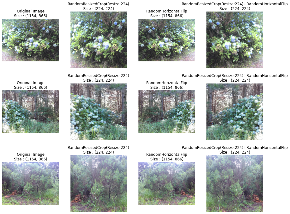
Train셋에 적용된 augmentation을 시각화하였습니다.
먼저 RandomResizedCrop을 통해 이미지를 scale범위 내의 비율로 랜덤하게 크롭한 후, size(224,224)로 크기를 조정했습니다. 그 다음 RandomHorizontalFlip으로 랜덤하게 좌우반전을 주었습니다.
2. Augmentation 확인하기(Valid)
Valid 데이터에 적용된 augmentation을 시각화했습니다.
1 | |
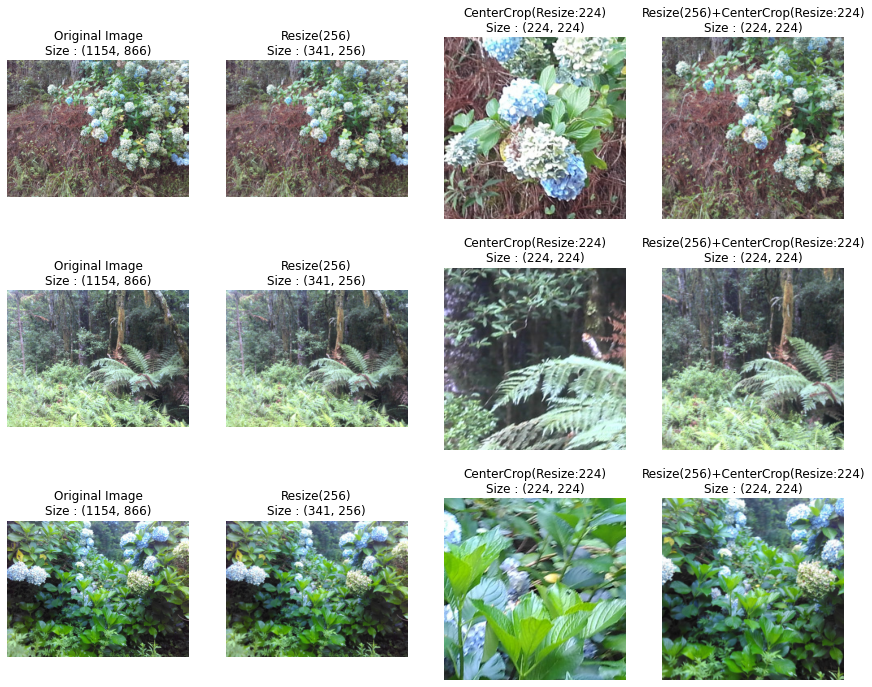
Valid 데이터에는 Resize 와 CenterCrop이 적용되었습니다.
Resize에서는 가로세로 비율을 유지하며 이미지 크기를 조정하였습니다. Invasive 대회의 데이터셋의 이미지들은 주로 중앙쪽에 주요 정보(침입종 식물)가 분포되어 있었습니다.
이러한 점을 이용하여 CenterCrop으로 중간 부분 위주로 이미지를 잘라내어 모델이 주요한 정보에 더욱 집중하여 학습할 수 있도록 하였습니다.
학습 준비
모델, Optimizer, Criterion
모델은 resnet18을 사용했습니다. 이진 분류이므로, num_classes를 2로 설정합니다.
Criterion은 CrossEntropyLoss, Optimizer은 Adam을 사용합니다.
1 | |
1 | |
한개의 배치에 대해 모델 성능 확인
전체 데이터를 학습하기 전, 우선 하나의 배치에 대해서 모델의 학습이 잘 이루어지는 확인합니다. 전체 데이터를 학습하게 되면, 모델이 잘 훈련되고 있는지 확인하기까지 시간이 많이 소요되므로 먼저 일부 데이터에 대해서만 학습을 진행해봅니다.
아래 출력되는 loss값을 보면, 모델 학습이 잘 이루어진 것을 확인할 수 있습니다.
1 | |
1 | |
Cut Mix
Cut Mix 설명
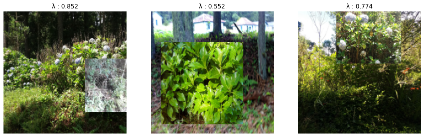
Cut mix은 주어진 이미지에 대해서 랜덤하게 패치를 만들어내어 다른 이미지에 합성하는 augmentation 기법 중 하나입니다.
Cut mix의 예시는 아래 4.결과에서 확인할 수 있습니다.
rand_bbox 함수는 패치를 생성하는 코드입니다. 주어진 이미지 크기 내에서, 랜덤하게 패치를 만들어내고 이에 대한 좌표를 반환하는 함수입니다.
패치의 폭과 넓이는, 주어진 이미지의 폭과 넓이에 np.sqrt(1-lam)을 곱하여 얻게 됩니다. 여기서 lam은 베타분포에서 랜덤하게 얻은 값입니다. 이렇게 얻어낸 패치 부분을, 랜덤하게 섞은 X(input)값들의 패치 부분으로 교체합니다.
이때 합성된 이미지의 레이블은, 합성된 전체 이미지에서 각각의 이미지가 차지하는 면적 비율만큼(lam)을 더한 값이 됩니다.
y = λ x invasive + (1-λ) x non-invasive
자세한 코드 설명은 아래에 있습니다.
이러한 cut mix 기법은 모델이 본 적이 없는 데이터에 대해서도 robust하게 예측할 수 있도록 도움을 줄 수 있습니다.
1 | |
Cut Mix 적용 과정
1. 배치 내의 데이터 셔플
데이터 로더에서 배치별로 데이터가 불러와지면, torch.randperm함수를 사용하여 인덱스를 랜덤하게 셔플합니다.
처음 람다값은 베타 분포에서 랜덤하게 가져옵니다.
1 | |
1 | |
2. 패치 부분 교체하기
기존 이미지의 패치 부분을, rand_index를 통해 셔플된 이미지들의 패치로 채워 넣습니다.
1 | |
3. 람다 조정하기
픽셀 비율과 정확히 일치하도록 람다를 조정합니다.
lam은 이후 loss값을 계산하는데 사용됩니다.
1 | |
1 | |
4. 결과
섞인 이미지를 볼 수 있습니다.
1 | |
1 | |
Cut Mix 결과 이미지
1 | |
모델 학습
Validation 함수
대회의 평가 지표가 area under the ROC curve이므로, validation 함수에서 AUC가 계산되도록 하였습니다.
1 | |
Train 함수
cut mix를 적용한 모델 훈련 코드입니다.
스케줄러는 ReduceLROnPlateau을 사용하였습니다.
val_loss가 가장 낮은 모델만 저장되도록 하였습니다.
1 | |
Fold 없이 단일 모델 학습
150개 데이터에 대해서 코드에 이상이 없는지 빠르게 실험해봤습니다.
1 | |
1 | |
5-Fold 학습
5번의 교차 검증 및 학습을 진행합니다. 각 교차 검증에서 가장 낮은 val_loss의 모델을 저장합니다. 이후 test 데이터 예측 시, 5개의 모델의 예측 결과를 voting을 통해 앙상블할 수 있습니다.
1 | |
1 | |
.
.
.
참고 자료
Invasive Hydrangeas : http://jenmenke.com/who-knew-hydrangeas-were-invasive/
CutMix Code(clovaai) : https://github.com/clovaai/CutMix-PyTorch
CutMix 설명 - 이유한님 : https://github.com/kaggler-tv/codes/blob/master/cutmix/cutmix.ipynb