대회 소개
National Data Science Bowl
Predict ocean health, one plankton at a time
https://www.kaggle.com/c/datasciencebowl
Description
Plankton are critically important to our ecosystem, accounting for more than half the primary productivity on earth and nearly half the total carbon fixed in the global carbon cycle. They form the foundation of aquatic food webs including those of large, important fisheries. Loss of plankton populations could result in ecological upheaval as well as negative societal impacts, particularly in indigenous cultures and the developing world. Plankton’s global significance makes their population levels an ideal measure of the health of the world’s oceans and ecosystems.
Traditional methods for measuring and monitoring plankton populations are time consuming and cannot scale to the granularity or scope necessary for large-scale studies. Improved approaches are needed. One such approach is through the use of an underwater imagery sensor. This towed, underwater camera system captures microscopic, high-resolution images over large study areas. The images can then be analyzed to assess species populations and distributions.
Manual analysis of the imagery is infeasible – it would take a year or more to manually analyze the imagery volume captured in a single day. Automated image classification using machine learning tools is an alternative to the manual approach. Analytics will allow analysis at speeds and scales previously thought impossible. The automated system will have broad applications for assessment of ocean and ecosystem health.
The National Data Science Bowl challenges you to build an algorithm to automate the image identification process. Scientists at the Hatfield Marine Science Center and beyond will use the algorithms you create to study marine food webs, fisheries, ocean conservation, and more. This is your chance to contribute to the health of the world’s oceans, one plankton at a time.
1 | |
1 | |
데이터 불러오기
- train, test 데이터가 zip으로 압축되어 있으므로 먼저 압축을 풀어주자.
1 | |
Train Dataset
- Train 데이터프레임을 만들어 주기
1 | |
| path | image | label | |
|---|---|---|---|
| 0 | train/train/pteropod_theco_dev_seq/36451.jpg | 36451.jpg | pteropod_theco_dev_seq |
| 1 | train/train/pteropod_theco_dev_seq/44793.jpg | 44793.jpg | pteropod_theco_dev_seq |
| 2 | train/train/pteropod_theco_dev_seq/157712.jpg | 157712.jpg | pteropod_theco_dev_seq |
| 3 | train/train/pteropod_theco_dev_seq/4992.jpg | 4992.jpg | pteropod_theco_dev_seq |
| 4 | train/train/pteropod_theco_dev_seq/144126.jpg | 144126.jpg | pteropod_theco_dev_seq |
| ... | ... | ... | ... |
| 30331 | train/train/hydromedusae_shapeB/27912.jpg | 27912.jpg | hydromedusae_shapeB |
| 30332 | train/train/hydromedusae_shapeB/49210.jpg | 49210.jpg | hydromedusae_shapeB |
| 30333 | train/train/hydromedusae_shapeB/114615.jpg | 114615.jpg | hydromedusae_shapeB |
| 30334 | train/train/hydromedusae_shapeB/81391.jpg | 81391.jpg | hydromedusae_shapeB |
| 30335 | train/train/hydromedusae_shapeB/95843.jpg | 95843.jpg | hydromedusae_shapeB |
30336 rows × 3 columns
Test Dataset
- Test 데이터 프레임을 만들어 주기
1 | |
| path | image | |
|---|---|---|
| 0 | ./test/test/105188.jpg | 105188.jpg |
| 1 | ./test/test/27651.jpg | 27651.jpg |
| 2 | ./test/test/11940.jpg | 11940.jpg |
| 3 | ./test/test/87538.jpg | 87538.jpg |
| 4 | ./test/test/95396.jpg | 95396.jpg |
| ... | ... | ... |
| 130395 | ./test/test/34122.jpg | 34122.jpg |
| 130396 | ./test/test/88776.jpg | 88776.jpg |
| 130397 | ./test/test/78514.jpg | 78514.jpg |
| 130398 | ./test/test/1830.jpg | 1830.jpg |
| 130399 | ./test/test/8917.jpg | 8917.jpg |
130400 rows × 2 columns
데이터 확인하기
- 이미지 모양 및 크기 확인
- class 개수 및 분포 확인
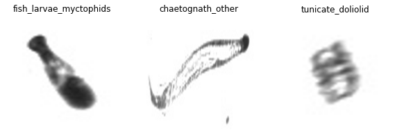
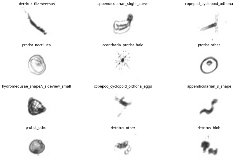
이미지 확인하기
1 | |
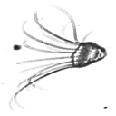
샘플 이미지 사이즈 확인하기
1 | |
1 | |
Train Dataset 이미지들의 평균 너비 및 높이
1 | |
1 | |
Label의 분포
1 | |
1 | |
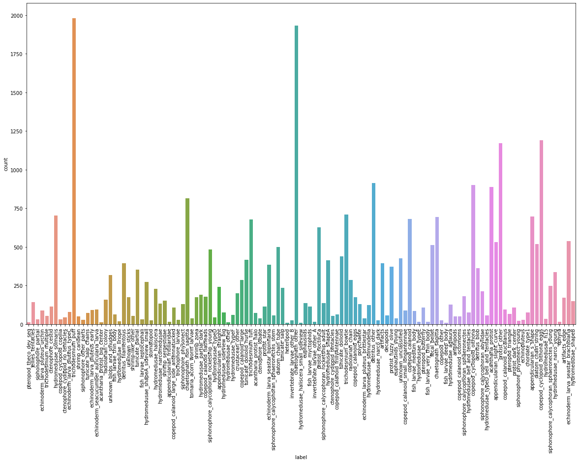
- 각
label별로 데이터의 분포가 다르다.
Test Dataset 전처리
1 | |
1 | |
교차 검증으로 모델 학습하기
1 | |
1 | |
1 | |
제출
- sampleSubmission.csv를 열어서 column의 순서를 확인해보면, 알파벳 순서로 들어가 있지 않다.
- result 칼럼의 순서와도 맞지 않으니, 이런 겨웅 직접 제출 파일을 만드는 것이 더 쉽다.
1 | |
| image | acantharia_protist_big_center | acantharia_protist_halo | acantharia_protist | amphipods | appendicularian_fritillaridae | appendicularian_s_shape | appendicularian_slight_curve | appendicularian_straight | artifacts_edge | ... | trichodesmium_tuft | trochophore_larvae | tunicate_doliolid_nurse | tunicate_doliolid | tunicate_partial | tunicate_salp_chains | tunicate_salp | unknown_blobs_and_smudges | unknown_sticks | unknown_unclassified | |
|---|---|---|---|---|---|---|---|---|---|---|---|---|---|---|---|---|---|---|---|---|---|
| 0 | 1.jpg | 0.008264 | 0.008264 | 0.008264 | 0.008264 | 0.008264 | 0.008264 | 0.008264 | 0.008264 | 0.008264 | ... | 0.008264 | 0.008264 | 0.008264 | 0.008264 | 0.008264 | 0.008264 | 0.008264 | 0.008264 | 0.008264 | 0.008264 |
| 1 | 10.jpg | 0.008264 | 0.008264 | 0.008264 | 0.008264 | 0.008264 | 0.008264 | 0.008264 | 0.008264 | 0.008264 | ... | 0.008264 | 0.008264 | 0.008264 | 0.008264 | 0.008264 | 0.008264 | 0.008264 | 0.008264 | 0.008264 | 0.008264 |
| 2 | 100.jpg | 0.008264 | 0.008264 | 0.008264 | 0.008264 | 0.008264 | 0.008264 | 0.008264 | 0.008264 | 0.008264 | ... | 0.008264 | 0.008264 | 0.008264 | 0.008264 | 0.008264 | 0.008264 | 0.008264 | 0.008264 | 0.008264 | 0.008264 |
| 3 | 1000.jpg | 0.008264 | 0.008264 | 0.008264 | 0.008264 | 0.008264 | 0.008264 | 0.008264 | 0.008264 | 0.008264 | ... | 0.008264 | 0.008264 | 0.008264 | 0.008264 | 0.008264 | 0.008264 | 0.008264 | 0.008264 | 0.008264 | 0.008264 |
| 4 | 10000.jpg | 0.008264 | 0.008264 | 0.008264 | 0.008264 | 0.008264 | 0.008264 | 0.008264 | 0.008264 | 0.008264 | ... | 0.008264 | 0.008264 | 0.008264 | 0.008264 | 0.008264 | 0.008264 | 0.008264 | 0.008264 | 0.008264 | 0.008264 |
| ... | ... | ... | ... | ... | ... | ... | ... | ... | ... | ... | ... | ... | ... | ... | ... | ... | ... | ... | ... | ... | ... |
| 130395 | 99994.jpg | 0.008264 | 0.008264 | 0.008264 | 0.008264 | 0.008264 | 0.008264 | 0.008264 | 0.008264 | 0.008264 | ... | 0.008264 | 0.008264 | 0.008264 | 0.008264 | 0.008264 | 0.008264 | 0.008264 | 0.008264 | 0.008264 | 0.008264 |
| 130396 | 99995.jpg | 0.008264 | 0.008264 | 0.008264 | 0.008264 | 0.008264 | 0.008264 | 0.008264 | 0.008264 | 0.008264 | ... | 0.008264 | 0.008264 | 0.008264 | 0.008264 | 0.008264 | 0.008264 | 0.008264 | 0.008264 | 0.008264 | 0.008264 |
| 130397 | 99996.jpg | 0.008264 | 0.008264 | 0.008264 | 0.008264 | 0.008264 | 0.008264 | 0.008264 | 0.008264 | 0.008264 | ... | 0.008264 | 0.008264 | 0.008264 | 0.008264 | 0.008264 | 0.008264 | 0.008264 | 0.008264 | 0.008264 | 0.008264 |
| 130398 | 99997.jpg | 0.008264 | 0.008264 | 0.008264 | 0.008264 | 0.008264 | 0.008264 | 0.008264 | 0.008264 | 0.008264 | ... | 0.008264 | 0.008264 | 0.008264 | 0.008264 | 0.008264 | 0.008264 | 0.008264 | 0.008264 | 0.008264 | 0.008264 |
| 130399 | 99999.jpg | 0.008264 | 0.008264 | 0.008264 | 0.008264 | 0.008264 | 0.008264 | 0.008264 | 0.008264 | 0.008264 | ... | 0.008264 | 0.008264 | 0.008264 | 0.008264 | 0.008264 | 0.008264 | 0.008264 | 0.008264 | 0.008264 | 0.008264 |
130400 rows × 122 columns
1 | |
1 | |
1 | |
| image | acantharia_protist | acantharia_protist_big_center | acantharia_protist_halo | amphipods | appendicularian_fritillaridae | appendicularian_s_shape | appendicularian_slight_curve | appendicularian_straight | artifacts | ... | trichodesmium_tuft | trochophore_larvae | tunicate_doliolid | tunicate_doliolid_nurse | tunicate_partial | tunicate_salp | tunicate_salp_chains | unknown_blobs_and_smudges | unknown_sticks | unknown_unclassified | |
|---|---|---|---|---|---|---|---|---|---|---|---|---|---|---|---|---|---|---|---|---|---|
| 0 | 105188.jpg | 3.407894e-05 | 5.234519e-07 | 4.727002e-07 | 2.523708e-05 | 6.414000e-07 | 1.429394e-04 | 7.389794e-05 | 2.510147e-05 | 8.997078e-08 | ... | 2.137576e-05 | 2.115729e-06 | 1.604188e-06 | 8.190606e-06 | 1.233781e-06 | 2.818242e-06 | 1.334955e-06 | 0.000023 | 7.377646e-05 | 0.000072 |
| 1 | 27651.jpg | 2.613361e-06 | 2.237140e-07 | 1.978252e-06 | 6.420553e-07 | 1.818773e-06 | 1.416835e-05 | 8.689414e-06 | 2.637850e-07 | 2.187041e-08 | ... | 2.810447e-07 | 9.286011e-07 | 8.374320e-06 | 2.925759e-06 | 2.006822e-07 | 2.315101e-07 | 7.389501e-07 | 0.000014 | 2.626070e-06 | 0.000423 |
| 2 | 11940.jpg | 6.104551e-06 | 2.521627e-06 | 2.513692e-07 | 4.636616e-05 | 2.085026e-06 | 1.489576e-05 | 8.225787e-05 | 1.137621e-05 | 3.021312e-07 | ... | 1.476521e-05 | 7.298316e-07 | 1.122896e-06 | 1.197497e-04 | 4.583527e-07 | 1.900000e-05 | 4.955790e-07 | 0.000482 | 3.988420e-05 | 0.002802 |
| 3 | 87538.jpg | 1.197881e-05 | 4.275779e-06 | 1.933437e-05 | 3.641628e-03 | 1.369998e-03 | 2.135313e-04 | 4.967969e-04 | 7.344080e-04 | 8.830065e-06 | ... | 1.323840e-01 | 8.188009e-06 | 6.234657e-04 | 2.646256e-04 | 5.426758e-05 | 1.694718e-03 | 1.481177e-05 | 0.000878 | 4.522099e-02 | 0.106003 |
| 4 | 95396.jpg | 1.079931e-07 | 1.477846e-06 | 4.025902e-07 | 9.353130e-05 | 6.802826e-07 | 3.575570e-06 | 4.541085e-07 | 1.869251e-07 | 2.157424e-07 | ... | 3.714577e-06 | 4.525396e-07 | 1.575890e-07 | 7.061017e-07 | 1.216337e-06 | 4.131224e-07 | 3.218001e-07 | 0.000011 | 8.910469e-07 | 0.000015 |
| ... | ... | ... | ... | ... | ... | ... | ... | ... | ... | ... | ... | ... | ... | ... | ... | ... | ... | ... | ... | ... | ... |
| 130395 | 34122.jpg | 9.404398e-06 | 4.410570e-06 | 1.469415e-05 | 4.892956e-04 | 4.235670e-04 | 7.620276e-04 | 7.704680e-05 | 4.103683e-05 | 1.476081e-05 | ... | 1.900832e-04 | 1.661727e-05 | 9.112542e-02 | 4.120418e-04 | 3.442946e-04 | 3.249257e-04 | 1.036034e-05 | 0.033025 | 1.140596e-05 | 0.008211 |
| 130396 | 88776.jpg | 1.188530e-04 | 3.108746e-06 | 7.981415e-06 | 2.125595e-07 | 5.005016e-08 | 5.221577e-07 | 6.974371e-07 | 1.526524e-06 | 1.525192e-05 | ... | 7.819511e-01 | 6.797829e-07 | 2.360160e-07 | 1.453742e-07 | 5.104931e-06 | 3.599948e-06 | 5.606108e-07 | 0.000010 | 1.053775e-04 | 0.000017 |
| 130397 | 78514.jpg | 3.513707e-06 | 1.072021e-07 | 6.263767e-07 | 2.130197e-07 | 8.390234e-07 | 3.240724e-05 | 1.973183e-04 | 1.500386e-04 | 1.360382e-08 | ... | 1.262665e-07 | 2.861952e-08 | 2.094702e-04 | 1.114861e-06 | 8.004471e-07 | 1.075251e-05 | 1.032177e-07 | 0.000038 | 1.695668e-06 | 0.000293 |
| 130398 | 1830.jpg | 2.687246e-08 | 6.054729e-10 | 1.001864e-07 | 2.510690e-08 | 9.267259e-09 | 2.659469e-08 | 6.407049e-08 | 6.902572e-08 | 9.994848e-01 | ... | 1.325866e-07 | 2.992527e-09 | 6.681008e-08 | 9.846344e-09 | 9.125281e-08 | 4.204970e-09 | 2.354498e-08 | 0.000091 | 7.961059e-08 | 0.000001 |
| 130399 | 8917.jpg | 1.647273e-07 | 1.519561e-07 | 9.120576e-08 | 1.517367e-03 | 1.538393e-07 | 2.816295e-07 | 6.235562e-07 | 5.191119e-06 | 2.437675e-06 | ... | 7.615223e-07 | 3.302962e-06 | 1.213374e-02 | 8.384104e-01 | 9.281476e-05 | 2.865229e-03 | 1.414542e-05 | 0.000016 | 7.298431e-06 | 0.003105 |
130400 rows × 122 columns
1 | |
Evaluation : Log Loss 0.65988
순위 : 1,049 중 35등