대회 소개
대회 주소 : https://www.dacon.io/competitions/official/235626/overview/
1 | |
데이터 불러오기
1 | |
| digit | letter | 0 | 1 | 2 | 3 | 4 | 5 | 6 | 7 | 8 | 9 | 10 | 11 | 12 | 13 | 14 | 15 | 16 | 17 | 18 | 19 | 20 | 21 | 22 | 23 | 24 | 25 | 26 | 27 | 28 | 29 | 30 | 31 | 32 | 33 | 34 | 35 | 36 | 37 | ... | 744 | 745 | 746 | 747 | 748 | 749 | 750 | 751 | 752 | 753 | 754 | 755 | 756 | 757 | 758 | 759 | 760 | 761 | 762 | 763 | 764 | 765 | 766 | 767 | 768 | 769 | 770 | 771 | 772 | 773 | 774 | 775 | 776 | 777 | 778 | 779 | 780 | 781 | 782 | 783 | |
|---|---|---|---|---|---|---|---|---|---|---|---|---|---|---|---|---|---|---|---|---|---|---|---|---|---|---|---|---|---|---|---|---|---|---|---|---|---|---|---|---|---|---|---|---|---|---|---|---|---|---|---|---|---|---|---|---|---|---|---|---|---|---|---|---|---|---|---|---|---|---|---|---|---|---|---|---|---|---|---|---|---|
| id | |||||||||||||||||||||||||||||||||||||||||||||||||||||||||||||||||||||||||||||||||
| 1 | 5 | L | 1 | 1 | 1 | 4 | 3 | 0 | 0 | 4 | 4 | 3 | 0 | 4 | 3 | 3 | 3 | 4 | 4 | 0 | 0 | 1 | 1 | 3 | 4 | 0 | 4 | 2 | 0 | 4 | 0 | 1 | 3 | 1 | 0 | 4 | 1 | 1 | 3 | 1 | ... | 4 | 3 | 4 | 1 | 3 | 0 | 0 | 1 | 3 | 3 | 3 | 0 | 3 | 2 | 2 | 1 | 0 | 1 | 0 | 0 | 3 | 0 | 0 | 4 | 2 | 0 | 3 | 4 | 1 | 1 | 2 | 1 | 0 | 1 | 2 | 4 | 4 | 4 | 3 | 4 |
| 2 | 0 | B | 0 | 4 | 0 | 0 | 4 | 1 | 1 | 1 | 4 | 2 | 0 | 3 | 4 | 0 | 0 | 2 | 3 | 4 | 0 | 3 | 4 | 3 | 0 | 2 | 2 | 1 | 4 | 2 | 3 | 3 | 4 | 1 | 2 | 4 | 2 | 0 | 3 | 2 | ... | 4 | 2 | 3 | 0 | 0 | 0 | 0 | 4 | 3 | 2 | 2 | 4 | 2 | 1 | 1 | 1 | 3 | 3 | 1 | 2 | 4 | 4 | 4 | 2 | 2 | 4 | 4 | 0 | 4 | 2 | 0 | 3 | 0 | 1 | 4 | 1 | 4 | 2 | 1 | 2 |
| 3 | 4 | L | 1 | 1 | 2 | 2 | 1 | 1 | 1 | 0 | 2 | 1 | 3 | 2 | 2 | 2 | 4 | 1 | 1 | 4 | 1 | 0 | 1 | 3 | 4 | 2 | 2 | 2 | 4 | 1 | 1 | 2 | 0 | 3 | 0 | 2 | 3 | 4 | 0 | 1 | ... | 3 | 0 | 4 | 0 | 3 | 0 | 2 | 0 | 1 | 4 | 2 | 3 | 4 | 4 | 4 | 0 | 2 | 0 | 4 | 4 | 1 | 3 | 0 | 3 | 2 | 0 | 2 | 3 | 0 | 2 | 3 | 3 | 3 | 0 | 2 | 0 | 3 | 0 | 2 | 2 |
| 4 | 9 | D | 1 | 2 | 0 | 2 | 0 | 4 | 0 | 3 | 4 | 3 | 1 | 0 | 3 | 2 | 2 | 0 | 3 | 4 | 1 | 0 | 4 | 1 | 2 | 2 | 3 | 2 | 2 | 0 | 2 | 0 | 3 | 0 | 3 | 2 | 4 | 0 | 0 | 4 | ... | 0 | 3 | 0 | 1 | 4 | 1 | 3 | 1 | 2 | 1 | 1 | 1 | 2 | 2 | 2 | 4 | 3 | 4 | 3 | 0 | 4 | 1 | 2 | 4 | 1 | 4 | 0 | 1 | 0 | 4 | 3 | 3 | 2 | 0 | 1 | 4 | 0 | 0 | 1 | 1 |
| 5 | 6 | A | 3 | 0 | 2 | 4 | 0 | 3 | 0 | 4 | 2 | 4 | 2 | 1 | 4 | 1 | 1 | 4 | 4 | 0 | 2 | 3 | 4 | 4 | 3 | 3 | 3 | 3 | 4 | 1 | 0 | 3 | 0 | 3 | 0 | 0 | 0 | 1 | 1 | 2 | ... | 2 | 1 | 3 | 2 | 1 | 4 | 2 | 3 | 2 | 2 | 1 | 0 | 4 | 2 | 2 | 1 | 2 | 1 | 0 | 3 | 2 | 2 | 2 | 2 | 1 | 4 | 2 | 1 | 2 | 1 | 4 | 4 | 3 | 2 | 1 | 3 | 4 | 3 | 1 | 2 |
5 rows × 786 columns
1 | |
| letter | 0 | 1 | 2 | 3 | 4 | 5 | 6 | 7 | 8 | 9 | 10 | 11 | 12 | 13 | 14 | 15 | 16 | 17 | 18 | 19 | 20 | 21 | 22 | 23 | 24 | 25 | 26 | 27 | 28 | 29 | 30 | 31 | 32 | 33 | 34 | 35 | 36 | 37 | 38 | ... | 744 | 745 | 746 | 747 | 748 | 749 | 750 | 751 | 752 | 753 | 754 | 755 | 756 | 757 | 758 | 759 | 760 | 761 | 762 | 763 | 764 | 765 | 766 | 767 | 768 | 769 | 770 | 771 | 772 | 773 | 774 | 775 | 776 | 777 | 778 | 779 | 780 | 781 | 782 | 783 | |
|---|---|---|---|---|---|---|---|---|---|---|---|---|---|---|---|---|---|---|---|---|---|---|---|---|---|---|---|---|---|---|---|---|---|---|---|---|---|---|---|---|---|---|---|---|---|---|---|---|---|---|---|---|---|---|---|---|---|---|---|---|---|---|---|---|---|---|---|---|---|---|---|---|---|---|---|---|---|---|---|---|---|
| id | |||||||||||||||||||||||||||||||||||||||||||||||||||||||||||||||||||||||||||||||||
| 2049 | L | 0 | 4 | 0 | 2 | 4 | 2 | 3 | 1 | 0 | 0 | 1 | 0 | 1 | 3 | 4 | 4 | 0 | 0 | 2 | 4 | 4 | 1 | 3 | 3 | 2 | 2 | 4 | 1 | 0 | 1 | 2 | 2 | 1 | 2 | 2 | 1 | 4 | 0 | 4 | ... | 1 | 3 | 1 | 1 | 3 | 3 | 4 | 1 | 3 | 1 | 2 | 4 | 1 | 2 | 0 | 3 | 1 | 2 | 4 | 0 | 2 | 1 | 2 | 4 | 1 | 1 | 3 | 2 | 1 | 0 | 2 | 0 | 4 | 2 | 2 | 4 | 3 | 4 | 1 | 4 |
| 2050 | C | 4 | 1 | 4 | 0 | 1 | 1 | 0 | 2 | 2 | 1 | 0 | 3 | 0 | 1 | 1 | 4 | 1 | 2 | 0 | 2 | 2 | 0 | 4 | 3 | 4 | 0 | 2 | 4 | 4 | 2 | 1 | 2 | 4 | 0 | 4 | 2 | 0 | 2 | 3 | ... | 3 | 4 | 2 | 6 | 2 | 2 | 0 | 1 | 2 | 4 | 1 | 1 | 3 | 3 | 2 | 3 | 4 | 2 | 2 | 4 | 3 | 1 | 3 | 3 | 3 | 1 | 3 | 4 | 4 | 2 | 0 | 3 | 2 | 4 | 2 | 4 | 2 | 2 | 1 | 2 |
| 2051 | S | 0 | 4 | 0 | 1 | 3 | 2 | 3 | 0 | 2 | 1 | 2 | 0 | 1 | 0 | 3 | 0 | 1 | 4 | 3 | 0 | 0 | 3 | 0 | 4 | 1 | 0 | 3 | 2 | 0 | 4 | 1 | 2 | 0 | 0 | 1 | 3 | 0 | 2 | 1 | ... | 0 | 4 | 4 | 3 | 4 | 1 | 4 | 2 | 3 | 4 | 1 | 2 | 0 | 2 | 2 | 3 | 3 | 1 | 1 | 4 | 1 | 2 | 4 | 0 | 0 | 0 | 0 | 2 | 3 | 2 | 1 | 3 | 2 | 0 | 3 | 2 | 3 | 0 | 1 | 4 |
| 2052 | K | 2 | 1 | 3 | 3 | 3 | 4 | 3 | 0 | 0 | 2 | 3 | 2 | 3 | 4 | 4 | 4 | 0 | 1 | 4 | 2 | 2 | 0 | 1 | 4 | 3 | 1 | 3 | 0 | 2 | 3 | 2 | 4 | 3 | 1 | 1 | 4 | 0 | 0 | 3 | ... | 0 | 4 | 1 | 1 | 2 | 3 | 2 | 3 | 3 | 0 | 0 | 1 | 3 | 3 | 0 | 2 | 0 | 0 | 2 | 3 | 2 | 2 | 3 | 1 | 1 | 2 | 4 | 0 | 1 | 2 | 3 | 0 | 3 | 2 | 4 | 1 | 0 | 4 | 4 | 4 |
| 2053 | W | 1 | 0 | 1 | 1 | 2 | 2 | 1 | 4 | 1 | 1 | 4 | 3 | 4 | 1 | 2 | 1 | 4 | 3 | 3 | 4 | 0 | 4 | 4 | 2 | 0 | 0 | 0 | 0 | 3 | 4 | 0 | 1 | 4 | 2 | 2 | 2 | 1 | 4 | 4 | ... | 4 | 1 | 3 | 2 | 1 | 2 | 1 | 4 | 4 | 1 | 2 | 3 | 2 | 4 | 2 | 1 | 4 | 3 | 4 | 3 | 0 | 1 | 0 | 1 | 1 | 2 | 1 | 1 | 0 | 2 | 4 | 3 | 1 | 4 | 0 | 2 | 1 | 2 | 3 | 4 |
5 rows × 785 columns
- digit을 맞춰야 하는 대회입니다.
데이터 살피기
1 | |
1 | |
- 데이터 shape 확인하기
1 | |
1 | |
- 0~9 숫자 10개
- 알파벳 26개
1 | |
1 | |
- 숫자 맞춰야 하기 때문에 digit을 category형으로 바꿔야 합니다.
1 | |
1 | |
- 목적변수의 분포를 파악합니다.
- 클래스간 어느정도 균형을 이루고 있음을 알수 있습니다.
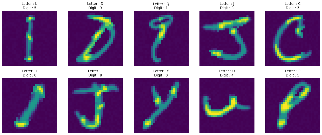
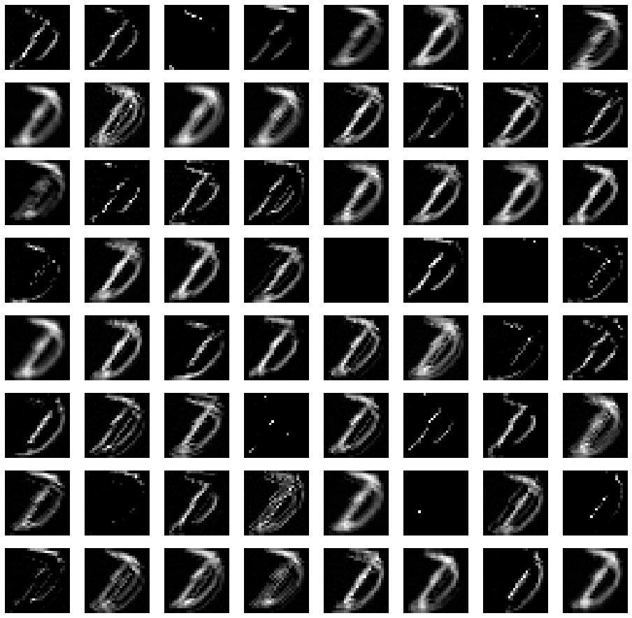
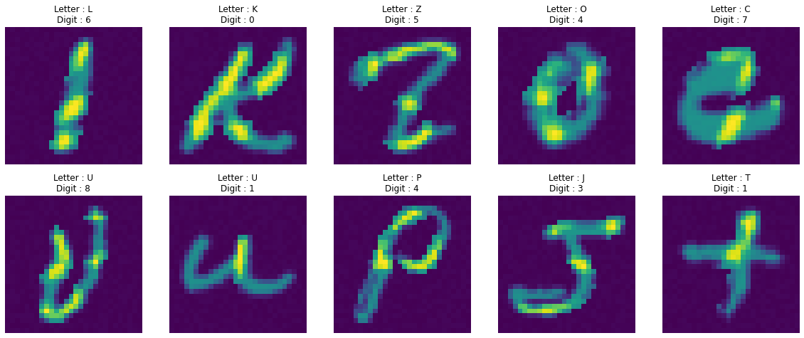
데이터 시각화
1 | |
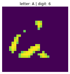
- 글자 속에 숫자가 숨겨져 있습니다.
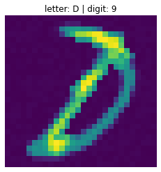
이미지 자세히 살펴보기
1 | |
1 |
|
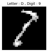
- D 속에 숨어있는 숫자 9
- 문자에 겹치는 숫자 부분만 표현된듯 합니다.
이미지에 Conv2D 적용하기
원본 이미지
1 | |
1 |
|
Conv2D 적용 후
1 | |
activation 적용 후
1 | |
MaxPooling2D 적용 후
1 | |
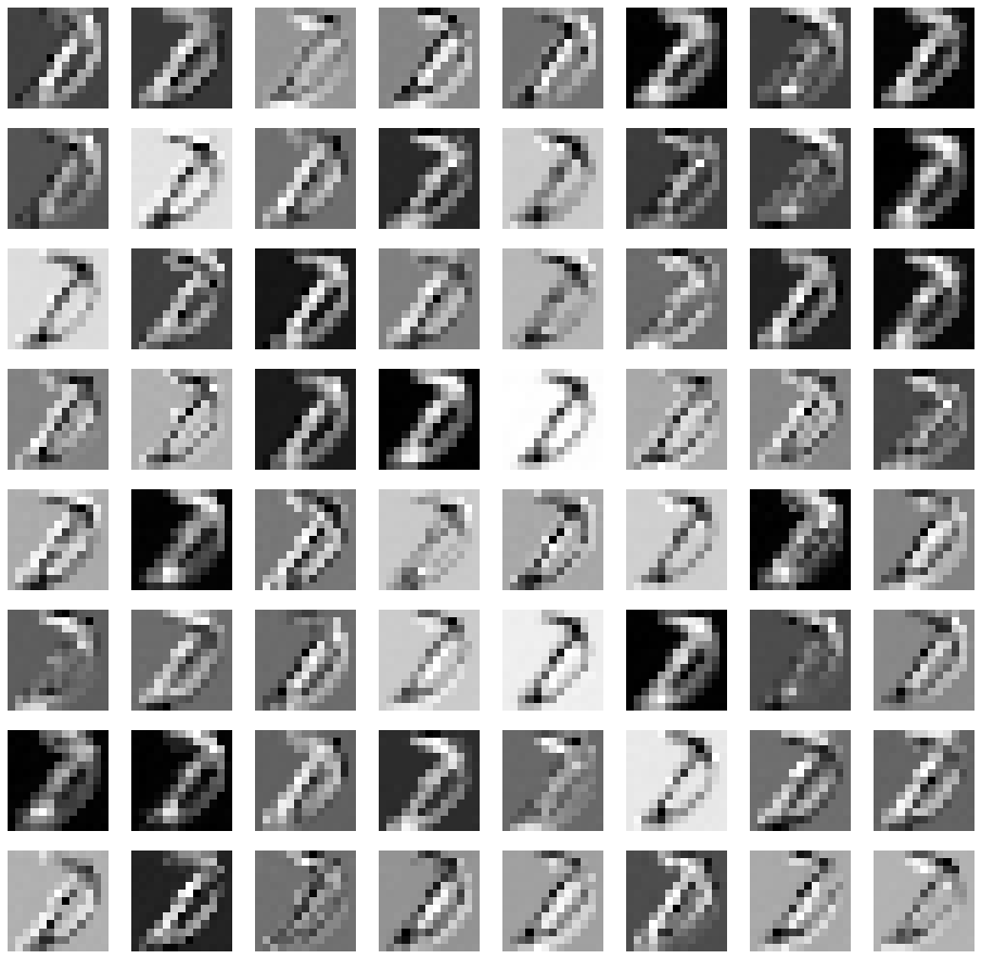
- Letter 부분이 지워지지 않고 그대로 학습됐습니다.
- Letter 부분 픽셀을 제거하고 학습하는 실험을 해봤습니다.
Letter와 숫자가 겹치는 Pixel 값만 나타내보기
1 | |
1 | |
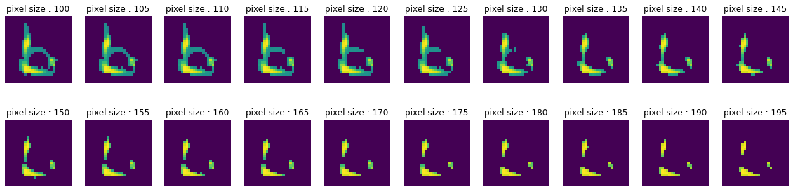
- Pixel값 약 140정도
- 많은 정보가 손실돼서 학습시 도움이 되지 않았습니다.
1 | |
1 |
|
Pixel값이 140 이상인 경우 Conv2D 적용
1 | |
1 |
|
1 | |
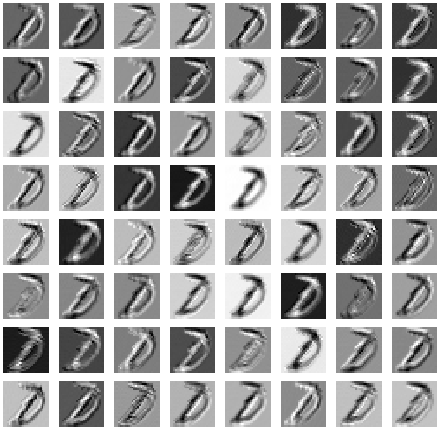
Data Augmentation
- train셋이 2048개로 class 개수에 비해 적습니다.
- 데이터 증강이 필요할 것 같습니다.
1 | |
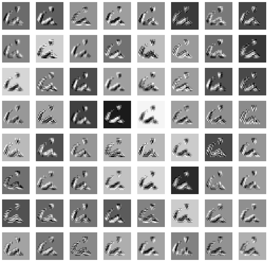
ImageDataGenerator로 Data Augmentation 후 모델 학습(모델 직접 구축)
1 | |
1 | |
최종 제출 코드
Train, Valid dataset 만들기
1 | |
모델 구축 및 학습
1 | |
학습 결과 시각화
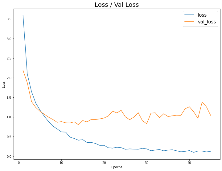
Loss / Val_loss 시각화
1 | |
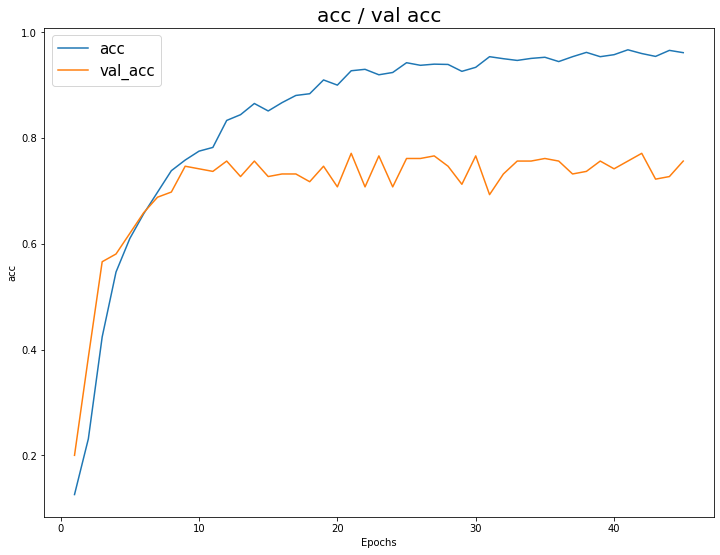
Accuracy / Val_Accuracy 시각화
1 | |
Test Dataset 전처리
1 | |
Test Dataset 예측 및 제출
1 | |
| digit | |
|---|---|
| id | |
| 2049 | 6 |
| 2050 | 8 |
| 2051 | 2 |
| 2052 | 0 |
| 2053 | 3 |
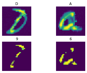
예측 결과 시각화
1 | |
- Letter는 주어진 값이고, 모델은 Digit을 예측합니다.